Part 0 — গাণিতিক ভিত্তি (Foundations) · Integrative Demos
পুরো "শূন্য → PhD" পরিসংখ্যান-যাত্রার ভিত্তি হলো ছয়টি গাণিতিক স্তম্ভ: set theory ও logic, combinatorics, differential calculus (optimization), integral calculus, linear algebra (eigen-decomposition), এবং computational thinking (vectorization)। এই module-এ প্রতিটি স্তম্ভের একটি flagship ধারণা চারভাবে দেখানো হয়েছে — (১) scratch (শুধু numpy), (২) library, (৩) empirical demonstration/"proof", (৪) visualization — সবই real open data (iris ও diabetes)-এর উপর, fixed seed 20260619 সহ। নিচের সব সংখ্যা executed notebook (notebooks/00-foundations.ipynb) থেকে নেওয়া।
চালানো:
cd notebooks && python3 -m nbconvert --to notebook --execute --inplace 00-foundations.ipynb --ExecutePreprocessor.timeout=600
0.1 — Sets, logic & proof: De Morgan on iris
ধারণা। যেকোনো property একটি index-set সংজ্ঞায়িত করে। iris-এর \(150\) rows-এর মধ্যে যেগুলোর sepal length তার median-এর চেয়ে বড়, তারা set \(A\); আর petal length median-এর চেয়ে বড় হলে set \(B\)। Set-এর সব operation — union (\(\cup\)), intersection (\(\cap\)), complement (\(\cdot^{c}\)), difference (\(\setminus\)) — boolean mask-এর উপর যথাক্রমে OR, AND, NOT, ও AND-NOT। এতে "logic" আর "set algebra" আসলে একই জিনিস।
Scratch-এর মূল ধারণা। প্রতিটি set = একটি length-\(150\) boolean mask (maskA = sl > median(sl))। Union maskA | maskB, intersection maskA & maskB, complement ~maskA, difference maskA & ~maskB। একটি mask-কে index-set-এ রূপান্তর: set(U[mask])। তারপর Python-এর built-in set operator (|, &, -)-এর সঙ্গে মিলিয়ে assert করা হয় — mask-algebra আর set-algebra একই ফল দেয়।
Demonstrated result (প্রমাণ)। iris-এ পাওয়া গেছে \(\lvert A\rvert=70,\ \lvert B\rvert=75,\ \lvert A\cup B\rvert=80,\ \lvert A\cap B\rvert=65\)। De Morgan's laws অক্ষরে-অক্ষরে যাচাই হয়েছে (set-সমতা হিসেবে):
আরও, চারটি disjoint region একসাথে universe-কে ঠিক ভাগ করে: \(\lvert A\cap B\rvert + \lvert A\setminus B\rvert + \lvert B\setminus A\rvert + \lvert (A\cup B)^{c}\rvert = 65+5+10+70 = 150 = \lvert U\rvert\)। এটাই দেখায় set operations গুলো সঙ্গতিপূর্ণ (consistent)।
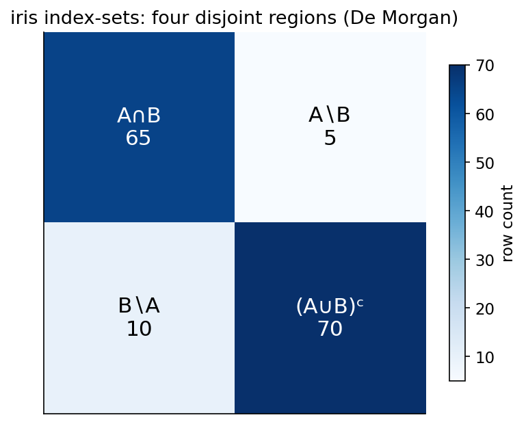
চিত্র: iris-এর চারটি disjoint region-এর row-count grid — \(\lvert A\cap B\rvert,\ \lvert A\setminus B\rvert,\ \lvert B\setminus A\rvert,\ \lvert (A\cup B)^{c}\rvert\)।
0.2 — Combinatorics & counting: Pascal's triangle
ধারণা। গণনার তিন ভিত্তি: factorial \(n! = \prod_{i=1}^{n} i\), permutation \(P(n,k)=\dfrac{n!}{(n-k)!}\) (ক্রম গুরুত্বপূর্ণ), এবং combination \(C(n,k)=\dfrac{n!}{k!\,(n-k)!}\) (ক্রম গুরুত্বহীন)। Combination-ই পরিসংখ্যানে binomial coefficient, তাই এটি Binomial distribution, Pascal's triangle, ও অসংখ্য identity-র মূল।
Scratch-এর মূল ধারণা। কোনো math.comb ছাড়া, শুধু integer arithmetic-এ। overflow ও fraction এড়াতে \(C(n,k)\)-কে ধাপে ধাপে বানানো হয়: symmetry দিয়ে \(k \leftarrow \min(k, n-k)\), তারপর num = num * (n-k+i) // i — প্রতি ধাপে exact integer division, যাতে মাঝপথেও সবসময় integer থাকে। \(P(n,k)\) হলো \(n\cdot(n-1)\cdots(n-k+1)\)-এর গুণফল।
Demonstrated result (প্রমাণ)। scratch-এর ফল math.comb, math.perm, math.factorial ও scipy.special.comb-এর সঙ্গে হুবহু মিলেছে (যেমন \(5!=120\), \(P(10,3)=720\), \(C(10,3)=120\), \(C(52,5)=2\,598\,960\))। দুটি ধ্রুপদী identity সব \(n\le 12\)-এর জন্য যাচাই হয়েছে:
Pascal's rule-ই Pascal's triangle বানানোর নিয়ম, আর row-sum দেখায় একটি \(n\)-সদস্যের set-এর মোট subset সংখ্যা \(2^{n}\)।
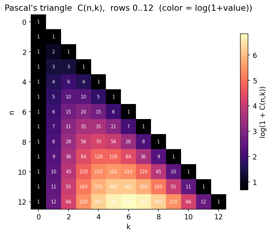
চিত্র: Pascal's triangle \(C(n,k)\), rows \(0\ldots12\); রং \(\log(1+C(n,k))\)-এর সমানুপাতিক।
0.3 — Calculus I: derivative & optimization (gradient descent)
ধারণা। Optimization-এর হৃদয় হলো derivative: minimum-এ gradient শূন্য। এখানে একটি feature \(x\) (diabetes-এর bmi, standardized) দিয়ে target \(y\)-কে সরলরেখায় fit করি, \(\hat y = w\,x + b\), এবং mean squared error \(L(w,b)=\frac1n\sum_i (w x_i + b - y_i)^2\) minimize করি। Gradient descent প্রতি ধাপে negative-gradient-এর দিকে ছোট পা (\(\text{lr}=0.1\)) ফেলে।
Scratch-এর মূল ধারণা। residual \(r_i = w x_i + b - y_i\) ধরে analytic gradient:
update rule: \(w \leftarrow w - \text{lr}\cdot \partial L/\partial w\), \(b \leftarrow b - \text{lr}\cdot \partial L/\partial b\); \((0,0)\) থেকে শুরু, \(2000\) iteration, প্রতি ধাপে loss track করা।
Demonstrated result (প্রমাণ)। GD-র শেষ ফল slope \(w = 0.586450\), intercept \(b \approx 0\) (standardize করায় প্রায় শূন্য), final MSE \(= 0.656076\)। এটি closed-form optimum-এর সঙ্গে হুবহু মিলেছে: normal equation (\(A^{\top}A\,\beta = A^{\top}y\)) দেয় slope \(= 0.586450\), আর np.polyfit-ও একই। loss একঘেয়েভাবে কমে ঠিক optimum-এ পৌঁছেছে (GD MSE \(-\) closed-form MSE gap \(= 0.00\))। বাড়তি insight (অন্তর্দৃষ্টি): standardized data-তে slope ঠিক Pearson correlation \(r = 0.586450\)-র সমান।
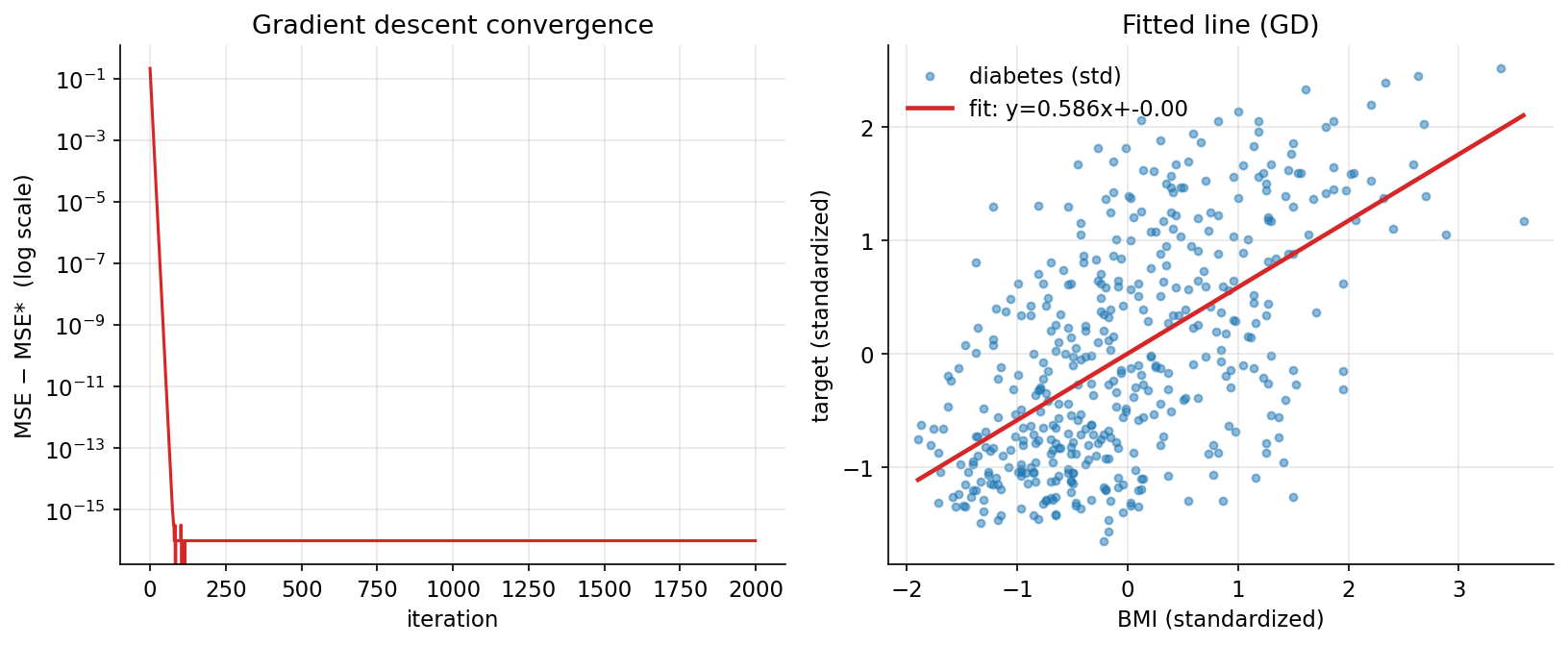
চিত্র (বাঁ): \(\text{MSE}-\text{MSE}^{*}\) log-scale-এ iteration-এর সাথে দ্রুত শূন্যে নামছে। (ডান): standardized BMI vs target scatter-এ GD-fitted রেখা।
0.4 — Calculus II: integration (trapezoid & Simpson)
ধারণা। নির্দিষ্ট integral \(\int_a^b f(x)\,dx\)-কে সংখ্যায় হিসাব করার দুই composite নিয়ম: trapezoid rule প্রতিটি উপ-অন্তরে \(f\)-কে সরলরেখা ধরে (error order \(h^{2}\)), আর Simpson's rule parabola ধরে (error order \(h^{4}\))। পরিসংখ্যানে এটি probability হিসাবের ভিত্তি — density-র নিচের ক্ষেত্রফলই probability।
Scratch-এর মূল ধারণা। \([a,b]\)-কে \(m\) সমান উপ-অন্তরে ভাগ; trapezoid: \(h\big(\tfrac12 y_0 + y_1 + \cdots + y_{m-1} + \tfrac12 y_m\big)\)। Simpson (even \(m\)): \(\tfrac{h}{3}\big(y_0 + y_m + 4\!\sum_{\text{odd}} y_i + 2\!\sum_{\text{even}} y_i\big)\)।
Demonstrated result (প্রমাণ)। standard normal pdf \(\phi\)-কে \([-1.96,\,1.96]\)-এ integrate করে পাওয়া গেছে \(0.950004\) (trapezoid ও Simpson উভয়েই) — অর্থাৎ চিরচেনা "\(95\%\) within \(\pm1.96\sigma\)"। আর \(\int_0^{40} e^{-x}dx = 1.000000\)। scipy-র quad দেয় \(\int\phi = 0.95000421\) ও \(\int_0^{\infty} e^{-x} = 1.0\), scratch Simpson-এর সঙ্গে মিলেছে। error convergence: \(h\) অর্ধেক করলে trapezoid error ভাগ হয় \(\approx 4\) গুণে (order \(h^{2}\)), আর Simpson error ভাগ হয় \(\approx 16\) গুণে (order \(h^{4}\)):
| \(m\) | trapezoid error | ratio | Simpson error | ratio |
|---|---|---|---|---|
| 8 | \(4.567\times10^{-3}\) | — | \(8.239\times10^{-5}\) | — |
| 16 | \(1.145\times10^{-3}\) | 3.99 | \(4.152\times10^{-6}\) | 19.84 |
| 32 | \(2.864\times10^{-4}\) | 4.00 | \(2.457\times10^{-7}\) | 16.90 |
| 64 | \(7.162\times10^{-5}\) | 4.00 | \(1.514\times10^{-8}\) | 16.22 |
| 128 | \(1.790\times10^{-5}\) | 4.00 | \(9.433\times10^{-10}\) | 16.06 |
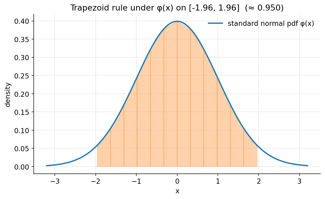
চিত্র: \([-1.96,\,1.96]\)-এ \(\phi(x)\)-এর নিচে trapezoid panel — নিচের ক্ষেত্রফল \(\approx 0.95\)।
0.5 — Linear algebra: eigen (power iteration → PCA)
ধারণা। iris-এর \(4\times4\) covariance matrix \(\Sigma\)-এর top eigenvector হলো সেই দিক যেখানে data-র variance সর্বোচ্চ — প্রথম principal component। এই একটি ধারণা থেকেই PCA, spectral methods, ও বহু multivariate কৌশল উৎপন্ন।
Scratch-এর মূল ধারণা। Power iteration: একটি random vector \(v\)-কে বারবার \(v \leftarrow \Sigma v / \lVert\Sigma v\rVert\) করলে সেটি top eigenvector-এ converge করে। eigenvalue পাওয়া যায় Rayleigh quotient \(\lambda = \dfrac{v^{\top}\Sigma v}{v^{\top}v}\) থেকে। (\(\Sigma\) centered data-র \(\tfrac{1}{n-1}X_c^{\top}X_c\)।)
Demonstrated result (প্রমাণ)। power iteration-এর top eigenvalue \(= 4.228242\), eigenvector \(\approx [\,0.361,\,-0.085,\,0.857,\,0.358\,]\) — np.linalg.eigh-এর top pair-এর সঙ্গে হুবহু মিলেছে (sign-aligned)। "max-variance" দাবি সরাসরি যাচাই: PC1-এ projection-এর variance \(= 4.228242\), ঠিক eigenvalue-র সমান, এবং \(5000\) random unit direction-এর মধ্যে সর্বোচ্চ variance \(= 4.207758 < 4.228242\) — কেউ PC1-কে হারাতে পারেনি। PC1 একাই মোট variance-এর \(92.46\%\) ব্যাখ্যা করে। Rayleigh quotient \(= 4.228242 =\) eigenvalue।
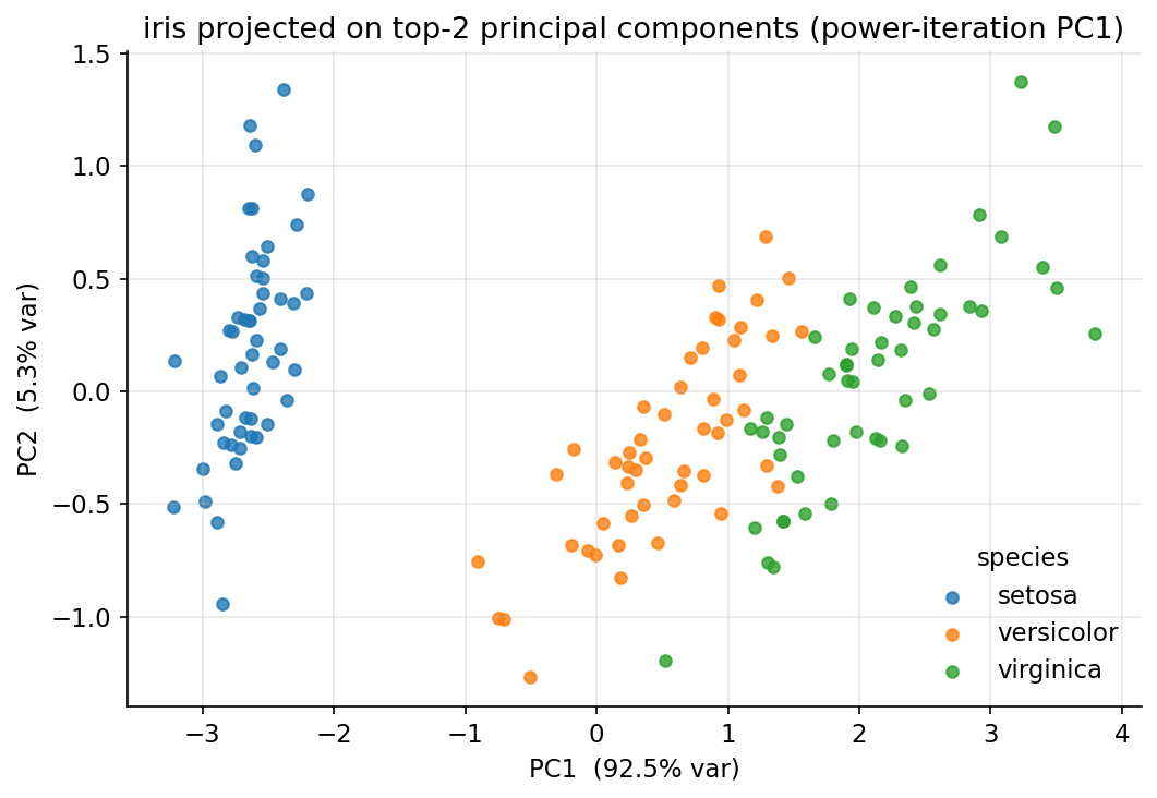
চিত্র: iris top-2 principal component-এ projected, species-অনুযায়ী রঙিন; PC1 (power-iteration) axis-এ তিন প্রজাতি স্পষ্ট আলাদা।
0.6 — Python/numpy: vectorization (broadcasting vs loop)
ধারণা। একই গণনা—iris feature-দের মধ্যে pairwise Euclidean distance—দুইভাবে করা যায়: (i) Python double loop, (ii) numpy broadcasting। ফল অবিকল একই, কিন্তু vectorized version অনেক দ্রুত। এটি computational statistics-এর ব্যবহারিক মেরুদণ্ড।
Scratch-এর মূল ধারণা। loop version: \(D_{ij}=\lVert x_i - x_j\rVert\) প্রতি জোড়ায় আলাদা। broadcasting version: X[:,None,:] - X[None,:,:] একবারে \((n,n,d)\) difference tensor বানায়, তারপর axis-2 বরাবর যোগ। ভিত্তিতে থাকা identity পুরো matrix-কে তিনটি matrix-op-এ নামায়:
Gram matrix \(G = XX^{\top}\) থেকে squared-distance \(= \operatorname{diag}(G)_i + \operatorname{diag}(G)_j - 2G_{ij}\)।
Demonstrated result (প্রমাণ)। \(60\times60\) distance-এ loop ও broadcasting-এর ফল bit-for-bit অভিন্ন, এবং দুটোই scipy.spatial.distance.cdist-এর সঙ্গে মিলেছে (max \(\lvert\Delta\rvert = 0\))। timing-এ broadcasting নাটকীয়ভাবে দ্রুত — এই run-এ loop \(\approx 4.31\) ms বনাম vectorized \(\approx 0.055\) ms, অর্থাৎ speedup \(\approx 79\times\) (নির্দিষ্ট সংখ্যা machine-নির্ভর, সাধারণত \(40\)–\(100\times\))। identity-ও যাচাই: Gram-matrix পথে গণিত distance broadcasting-এর সাথে মেলে (max \(\lvert\Delta\rvert = 6.67\times10^{-14}\), নিছক floating-point round-off)।
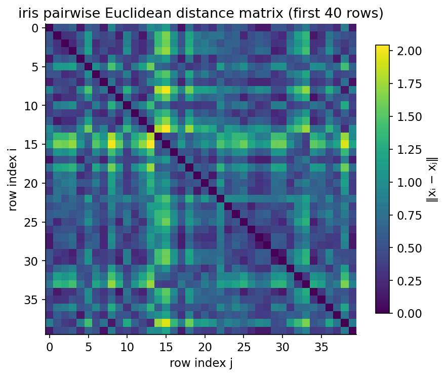
চিত্র: প্রথম \(40\) iris row-এর pairwise Euclidean distance matrix; block-structure প্রজাতি-গুচ্ছ দেখায়।
সারসংক্ষেপ (Part 0)
| ধারা | scratch ↔ library মিল | মূল প্রমাণিত ফল |
|---|---|---|
| 0.1 | mask-algebra == Python set |
De Morgan দুই সূত্রই সত্য; \(65+5+10+70=150\) |
| 0.2 | == math.comb/perm, scipy.comb |
Pascal rule ও \(\sum_k C(n,k)=2^n\) |
| 0.3 | GD == normal eq == polyfit |
slope \(0.586450\), gap \(=0\), slope \(=r\) |
| 0.4 | Simpson == scipy.quad |
\(\int\phi\approx0.95\), \(\int e^{-x}\approx1\); error \(h^2\) vs \(h^4\) |
| 0.5 | power-iter == eigh |
\(\lambda_1=4.2282\), PC1 \(=\) max-var \(=\) Rayleigh, \(92.46\%\) |
| 0.6 | loop == broadcast == cdist |
identity holds; \(\sim\!79\times\) speedup |
প্রতিটি ধারণা এখন চলমান, পুনরুৎপাদনযোগ্য কোডে বাঁধা — এই ভিত্তির উপরেই Parts I–VII দাঁড়াবে।