Part IV — পরিসংখ্যানিক inference (অনুমান) · Integrative Demos

Part IV পরিসংখ্যানের সেই স্তম্ভগুলো ধরে যেখানে সীমিত data থেকে অজানা parameter সম্পর্কে সিদ্ধান্ত নেওয়া হয়: sampling distribution, method of moments, maximum likelihood (MLE), estimator properties (bias/variance/MSE), Fisher information ও Cramér–Rao lower bound, confidence interval ও coverage, hypothesis testing ও power, likelihood-ratio/Wald/score triad, bootstrap/jackknife/permutation, এবং Bayesian inference। প্রতিটি ধারণা চারভাবে দেখানো — (b) scratch (শুধু numpy), (c) library check (scipy.stats/statsmodels), (d) demonstrate/"prove" (ছাপা real সংখ্যা), (e) visualization — সবই real open data (iris, breast_cancer, diabetes)-এর উপর, fixed seed 20260619 সহ। নিচের সব সংখ্যা executed notebook (notebooks/04-inference.ipynb) থেকে সরাসরি নেওয়া।

চালানো: cd notebooks && python3 -m nbconvert --to notebook --execute --inplace 04-inference.ipynb --ExecutePreprocessor.timeout=1200

---

4.1 — Sampling distributions (bootstrap sampling distribution of the median)

ধারণা। একটা statistic (এখানে median) নিজেই একটা random পরিমাণ — ভিন্ন sample দিলে ভিন্ন মান। তার সম্ভাব্য মানের বণ্টনকে বলে sampling distribution, আর তার standard deviation-কে বলে standard error (SE)। median-এর SE-এর সরল closed-form নেই, তাই bootstrap (মূল sample থেকে with-replacement বারবার resample করে statistic-এর বণ্টন গড়া) দিয়ে সেটা আঁকা হয়।

Scratch-এর মূল ধারণা। breast_cancer-এর mean radius (\(N=569\)) থেকে \(B=20{,}000\) বার full-size (\(n=N\)) with-replacement resample করে প্রতিটির median নেওয়া হয়; সেই \(B\)টি median-এর বণ্টনই sampling distribution, আর তাদের sd হলো SE।

Demonstrated result (প্রমাণ)। sample median \(\hat\theta=13.370000\); bootstrap medians-এর গড় \(=13.349259\), SE \(=0.159552\), bias estimate \(=-0.020741\)। \(95\%\) percentile CI \(=[13.0500,\ 13.6500]\) — sample median ধরে রাখে। raw feature-এর sd \(=3.5240\), কিন্তু SE(median) মাত্র \(0.1596\): অনুপাত \(\mathbf{22.09\times}\) — অর্থাৎ statistic একটা মাত্র datum-এর চেয়ে অনেক বেশি stable। scipy-র bootstrap SE-ও \(0.159552\) (হুবহু মেলে); rough asymptotic \(1/(2f(m)\sqrt n)=0.154656\) কাছাকাছি।

\[\operatorname{SE}(\text{median})=\operatorname{sd}\!\big(\hat\theta^{*(1)},\dots,\hat\theta^{*(B)}\big)=0.1596,\qquad \frac{\operatorname{sd}(x)}{\operatorname{SE}}=22.1.\]

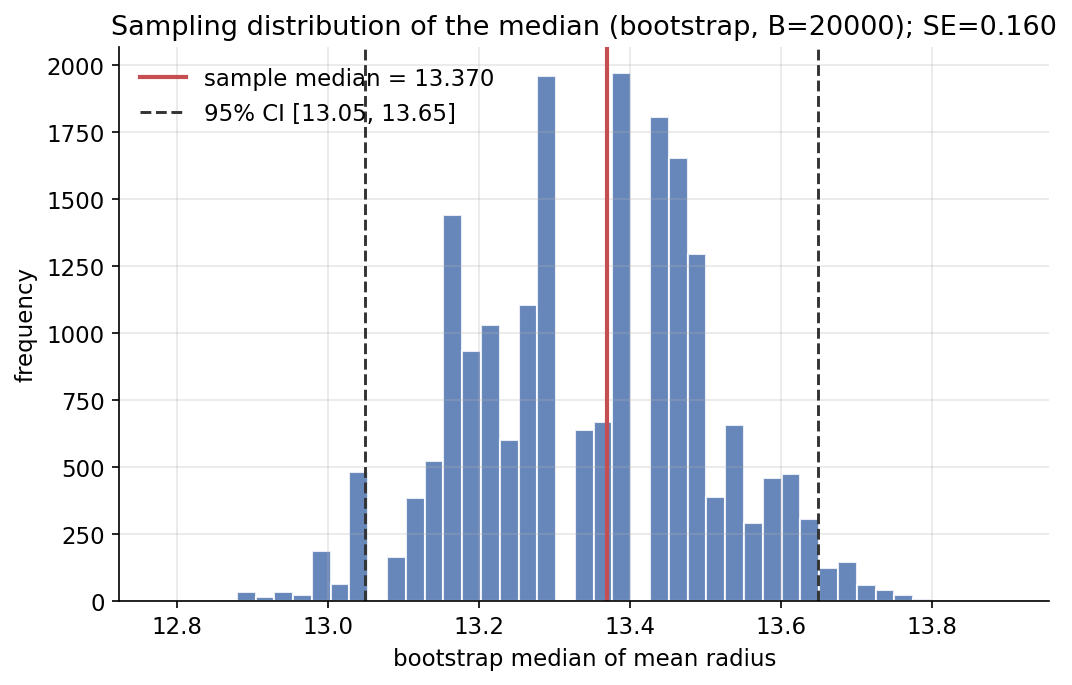
চিত্র: breast_cancer mean radius-এর median-এর bootstrap sampling distribution (\(B=20000\)), sample median ও \(95\%\) percentile CI চিহ্নিত।

---

4.2 — Method of moments (Gamma fit to a positive feature)

ধারণা। Method of moments (MoM) parameter বের করে theoretical moment-গুলোকে sample moment-এর সমান বসিয়ে। Gamma\((k,\theta)\)-এর mean \(=k\theta\), variance \(=k\theta^2\); তাই sample \(\bar x,s^2\) ম্যাচ করে shape \(k=\bar x^2/s^2\) এবং scale \(\theta=s^2/\bar x\) — মুহূর্তেই একটা estimate।

Scratch-এর মূল ধারণা। diabetes-এর bmi (strictly-positive-এ shift করা) থেকে \(\bar x,s^2\) নিয়ে \(k=\bar x^2/s^2,\ \theta=s^2/\bar x\) হিসাব; তারপর সেই Gamma-র pdf histogram-এর উপর বসানো।

Demonstrated result (প্রমাণ)। shifted bmi (\(n=442\)): sample mean \(=0.091275\), var \(=0.002262\) → MoM shape \(k=3.682381\), scale \(\theta=0.024787\)। moment-matching identity হুবহু ধরে: \(k\theta=0.09127530\) (\(=\) sample mean), \(k\theta^2=0.00226244\) (\(=\) sample var)। scipy-র gamma(k,\theta)-এর mean/var একই — দুটোই True। MoM-এর fit ভালো: KS statistic \(=0.0389,\ p=0.5038\) (data ও MoM Gamma আলাদা নয়)। তুলনায় MLE fit দেয় \(k=3.0385,\ \theta=0.0300\) — MoM ও MLE একই নয়, এটাই দুই পদ্ধতির স্বাভাবিক পার্থক্য।

\[k=\frac{\bar x^2}{s^2}=3.6824,\qquad \theta=\frac{s^2}{\bar x}=0.02479,\qquad k\theta=\bar x,\ \ k\theta^2=s^2\ \text{(হুবহু)}.\]

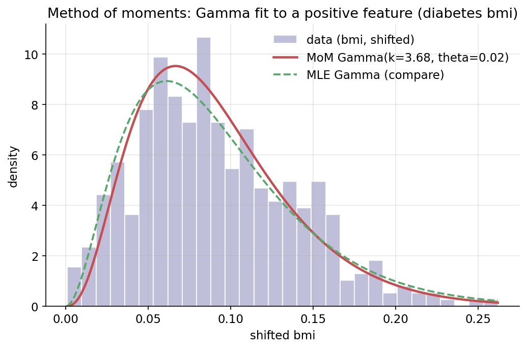
চিত্র: diabetes bmi-এর histogram-এর উপর MoM Gamma pdf (লাল) ও তুলনায় MLE Gamma (সবুজ ড্যাশ)।

---

4.3 — Maximum likelihood estimation (Normal ও Bernoulli)

ধারণা। MLE সেই parameter বেছে নেয় যেটা observed data-কে সবচেয়ে সম্ভাব্য করে — অর্থাৎ log-likelihood \(\ell(\theta)\) সর্বোচ্চ করে। Normal-এর closed form \(\hat\mu=\bar x,\ \hat\sigma^2=\frac1n\sum(x_i-\bar x)^2\) (ddof\(=0\)!); Bernoulli-এর \(\hat p=\bar x\)।

Scratch-এর মূল ধারণা। iris sepal length-এর Normal MLE (\(\bar x\), population variance); "sepal length \(>\) median" indicator-এর Bernoulli MLE (\(\hat p=\bar b\)); log-likelihood function হাতে লিখে তার শীর্ষ যাচাই।

Demonstrated result (প্রমাণ)। Normal (\(n=150\)): \(\hat\mu=5.843333,\ \hat\sigma^2=0.681122,\ \hat\sigma=0.825301\), max log-lik \(=-184.0398\)। scipy-র norm.fit হুবহু একই \(\mu,\sigma\) দেয় (দুটোই True)। Bernoulli: \(\hat p=0.466667\), grid-argmax \(=0.4666\) (closed form \(0.4667\)-এর সাথে মেলে)। MLE যে সত্যিই maximum তার প্রমাণ: \(\ell(\hat\mu-0.15)=\ell(\hat\mu+0.15)=-186.5173 < \ell(\hat\mu)=-184.0398\), এবং score \(\partial\ell/\partial\mu\big\rvert_{\hat\mu}=-7.30\times10^{-14}\approx 0\) (first-order condition)।

\[\hat\mu=\bar x=5.8433,\quad \hat\sigma^2=\tfrac1n\textstyle\sum(x_i-\bar x)^2=0.6811,\qquad \frac{\partial\ell}{\partial\mu}\Big\rvert_{\hat\mu}=0.\]

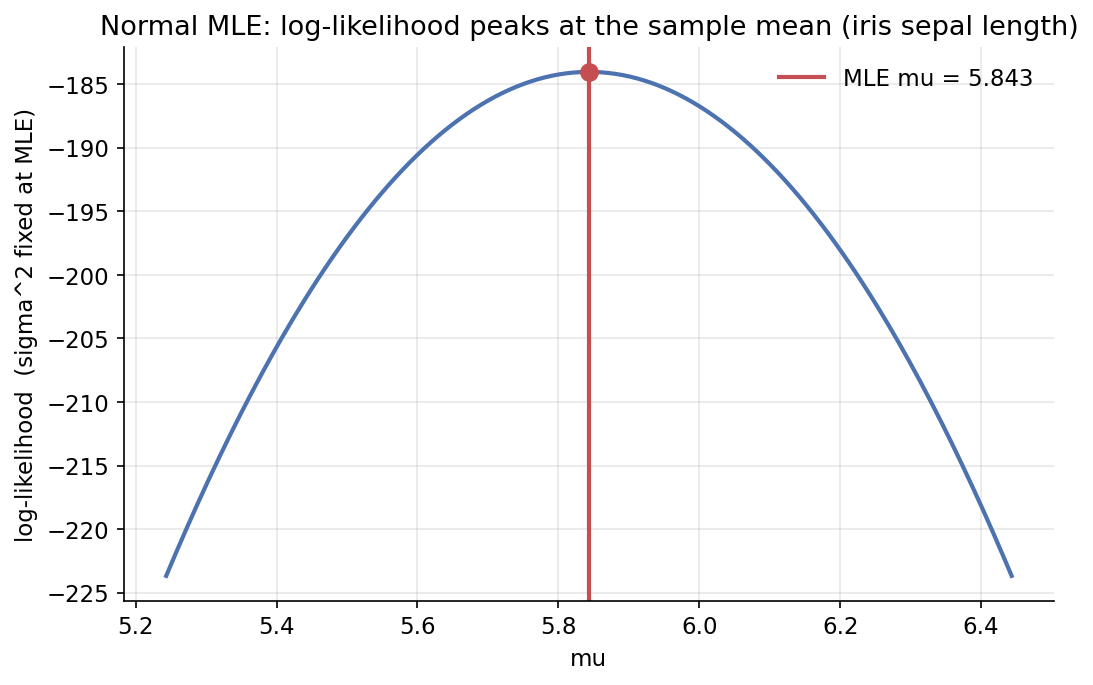
চিত্র: iris sepal length-এর Normal log-likelihood (\(\mu\)-এর ফাংশন, \(\sigma^2\) MLE-তে স্থির); শীর্ষ ঠিক sample mean-এ।

---

4.4 — Estimator properties (bias / variance / MSE of the sample variance)

ধারণা। estimator-এর গুণ মাপা হয় bias (\(E[\hat\theta]-\theta\)), variance, ও MSE \(=\) bias\(^2+\) variance দিয়ে। sample variance-এ \(\text{ddof}=0\) biased (নিচু), \(\text{ddof}=1\) unbiased; \(n\to\infty\)-এ দুটোরই MSE \(\to 0\) — consistent।

Scratch-এর মূল ধারণা। breast_cancer mean radius-কে "population" ধরে (\(\sigma^2=12.397094\)), প্রতিটি \(n\)-এ হাজার হাজার resample থেকে \(s^2_{\text{ddof}=0}\) ও \(s^2_{\text{ddof}=1}\)-এর bias/variance/MSE Monte-Carlo করে মাপা।

Demonstrated result (প্রমাণ)। \(n=10\)-এ: ddof\(=0\) bias \(=-1.35644\) (theory \(-\sigma^2/n=-1.23971\)-এর কাছাকাছি), ddof\(=1\) bias \(=-0.12970\) — অনেক ছোট। \(n\) বাড়লে ddof\(=1\)-এর \(\lvert\text{bias}\rvert\) থিতিয়ে যায় (\(n{=}20\!:+0.078,\ n{=}200\!:-0.017\)) এবং উভয়ের MSE \(\to 0\): ddof\(=1\) MSE \(102.03\ (n{=}5)\to 44.81\ (n{=}10)\to 2.27\ (n{=}200)\)। identity var(ddof=1)=var(ddof=0)·n/(n-1) হুবহু ধরে (True)।

\[E[s^2_{\text{ddof}=1}]=\sigma^2\ \text{(unbiased)},\qquad \operatorname{bias}(s^2_{\text{ddof}=0})\approx-\frac{\sigma^2}{n}\xrightarrow[n\to\infty]{}0.\]

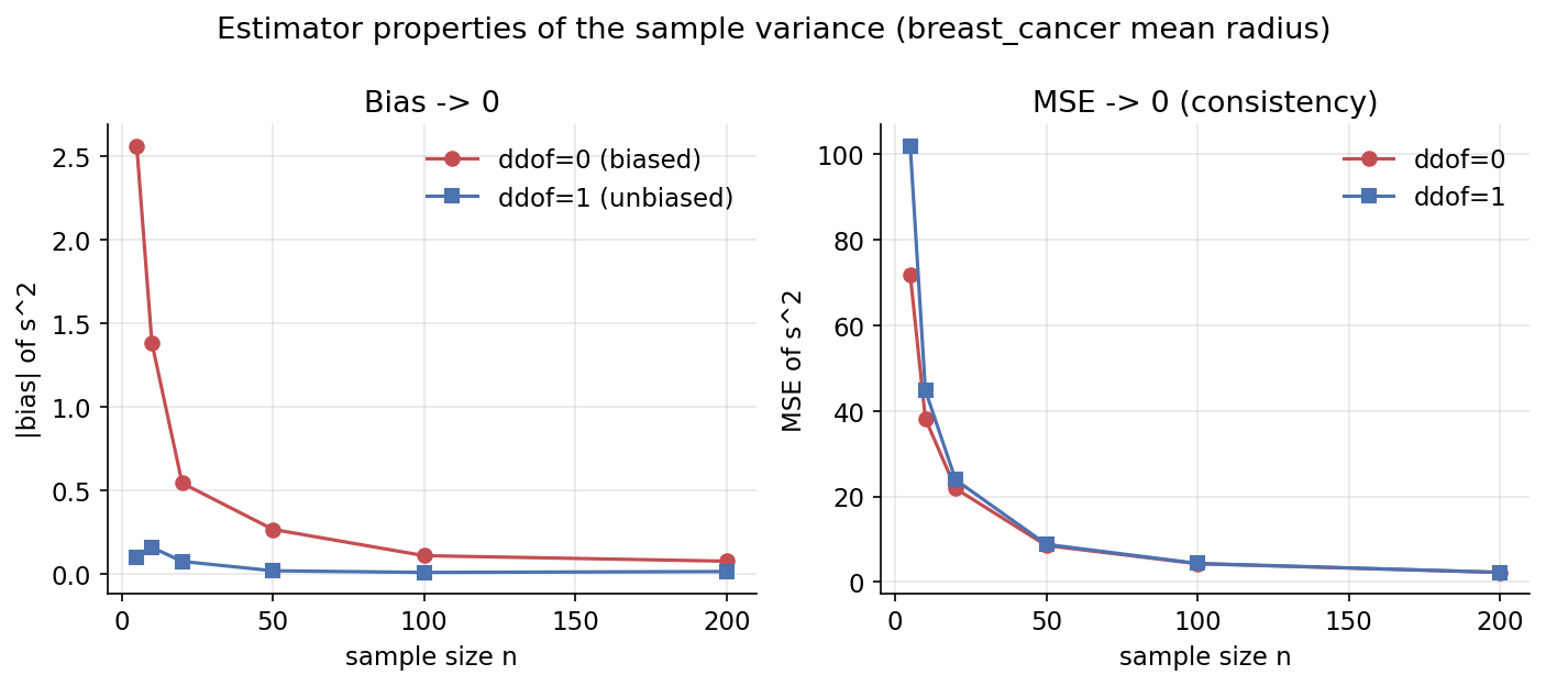
চিত্র: দুই panel — \(\lvert\text{bias}\rvert\) বনাম \(n\) (ddof\(=1\) প্রায় শূন্য), এবং MSE বনাম \(n\) (দুটোই \(\to 0\): consistency)।

---

4.5 — Fisher information ও Cramér–Rao lower bound

ধারণা। Fisher information \(I(\theta)=-E[\partial^2\ell/\partial\theta^2]\) মাপে data parameter সম্পর্কে কতটা তথ্য বহন করে। Normal mean-এর \(I(\mu)=n/\sigma^2\)। CRLB বলে যেকোনো unbiased estimator-এর variance \(\ge 1/I(\mu)=\sigma^2/n\); sample mean এই সীমা ছুঁয়ে ফেলে — তাই সে efficient।

Scratch-এর মূল ধারণা। iris petal length-কে population ধরে (\(\sigma^2=3.095503\)), \(n=25\)-এ \(I(\mu)=n/\sigma^2\) ও CRLB \(=\sigma^2/n\) হিসাব; তারপর \(40{,}000\) resample থেকে sample mean-এর empirical variance মেপে CRLB-এর সাথে অনুপাত।

Demonstrated result (প্রমাণ)। \(n=25\): \(I(\mu)=8.076233\), CRLB \(=0.123820\); empirical Var(sample mean) \(=0.123963\) → ratio \(=1.0012\approx 1\) (সীমা ছোঁয়)। \(1/I(\mu)=\text{CRLB}\) (True), এবং \(\sigma/\sqrt n=0.351881\) vs empirical sd \(0.352084\)। বিভিন্ন \(n\)-এ ratio প্রায় \(1\)-এই থাকে (\(n{=}10\!:0.990,\ n{=}50\!:1.003,\ n{=}200\!:1.002\)) — sample mean সর্বত্র efficient।

\[I(\mu)=\frac{n}{\sigma^2},\qquad \operatorname{Var}(\bar X)\ \ge\ \frac{1}{I(\mu)}=\frac{\sigma^2}{n}=\text{CRLB},\qquad \frac{\operatorname{Var}(\bar X)}{\text{CRLB}}=1.00.\]

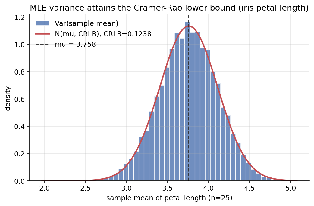
চিত্র: iris petal length-এর sample mean-এর sampling distribution (\(n=25\)), তার উপর \(N(\mu,\text{CRLB})\) — variance ঠিক CRLB।

---

4.6 — Confidence intervals (z · t · bootstrap) ও coverage

ধারণা। একটা CI এমন ব্যবধান যা বারবার sampling-এ প্রকৃত parameter-কে নির্দিষ্ট হারে (\(95\%\)) ভিতরে রাখে। জানা \(\sigma\)-তে z-interval \(\bar x\pm z_{.975}\sigma/\sqrt n\); অজানা \(\sigma\)-তে t-interval (Student-\(t\)); আর distribution-free bootstrap percentile interval। coverage simulation দেখায় সত্যিই \(\approx 95\%\) CI প্রকৃত mean ধরে।

Scratch-এর মূল ধারণা। iris setosa sepal length (\(n=50\))-এ \(\bar x,s\) থেকে z ও bootstrap CI; scipy দিয়ে t-critical। তারপর column-কে population ধরে \(5000\) বার \(n=30\) sample টেনে t-CI বানিয়ে গোনা কতবার প্রকৃত mean ভিতরে থাকে।

Demonstrated result (প্রমাণ)। \(\bar x=5.006000,\ s=0.352490,\ \text{SE}=0.049850\)। z \(95\%\) CI \(=[4.9083,5.1037]\); bootstrap \(=[4.9080,5.1040]\); t \(=[4.9058,5.1062]\) (scipy t.interval-এর সাথে হুবহু, True)। width: z\(=0.1954 <\) t\(=0.2004\) — t সঠিকভাবেই সামান্য চওড়া। coverage simulation: nominal \(95\%\)-এর বিপরীতে empirical coverage \(=\mathbf{0.9524}\)।

\[\bar x\pm t_{.975,\,n-1}\frac{s}{\sqrt n}=[4.906,\ 5.106],\qquad \text{empirical coverage}=95.24\%.\]

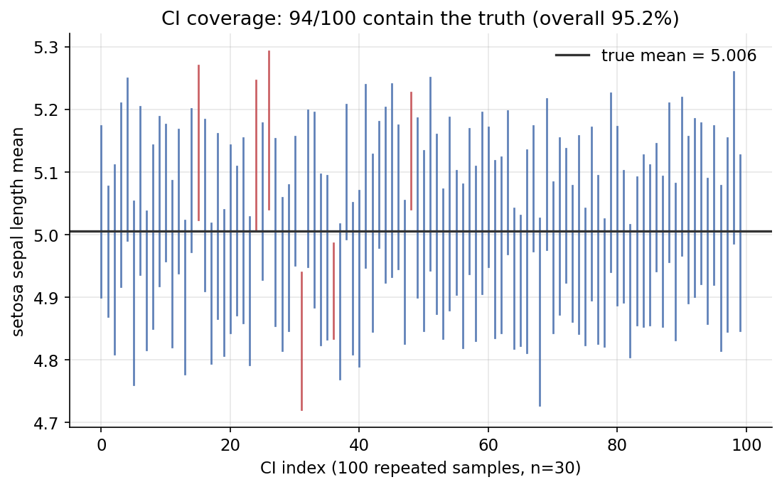
চিত্র: \(100\)টি পুনরাবৃত্ত t-CI (\(n=30\)); নীল CI প্রকৃত mean ধরে, লাল ধরে না — মোট \(\approx 95\%\) ধরে।

---

4.7 — Hypothesis testing (two-sample t-test · power · p-value distribution)

ধারণা। Hypothesis test নাল \(H_0\) (দুই প্রজাতির mean সমান) বনাম বিকল্পের বিরুদ্ধে data-র সাক্ষ্য ওজন করে। pooled two-sample t \(t=\dfrac{\bar x_1-\bar x_2}{\sqrt{s_p^2(1/n_1+1/n_2)}}\); ছোট p-value মানে \(H_0\)-এর অধীনে এমন চরম মান বিরল। power সত্য effect ধরার সম্ভাবনা; \(H_0\) সত্য হলে p-value Uniform(0,1)।

Scratch-এর মূল ধারণা। iris setosa বনাম versicolor sepal length-এ pooled \(s_p^2\), scratch \(t\) ও two-sided p (via \(t\)-CDF); noncentral-\(t\) দিয়ে effect size \(\delta\)-এর ফাংশনে power; আর label permutation করে \(H_0\)-এর অধীনে p-value-এর বণ্টন।

Demonstrated result (প্রমাণ)। setosa mean \(=5.0060\), versicolor \(=5.9360\) (\(n=50\) each), \(s_p^2=0.195341\), df\(=98\)। scratch \(t=-10.520986\), \(p=8.985\times10^{-18}\) — scipy ttest_ind-এর সাথে \(t\) ও \(p\) উভয়ে হুবহু (True) — প্রবল প্রমাণ যে mean আলাদা। power effect size-এ বাড়ে: \(\delta{=}0\!:0.0500\ (=\alpha),\ \delta{=}0.5\!:0.9365,\ \delta{=}1.0\!:1.0000\)। \(H_0\)-এর অধীনে p-value Uniform: mean \(p=0.4966\), frac \(p<0.05=0.0522\), KS-vs-Uniform \(p=0.0596\) (বড় \(\Rightarrow\) uniform)।

\[t=-10.52,\quad p\approx 9\times10^{-18};\qquad \text{power}(\delta{=}0.5)=0.94;\qquad p\mid H_0\sim \mathrm{Uniform}(0,1).\]

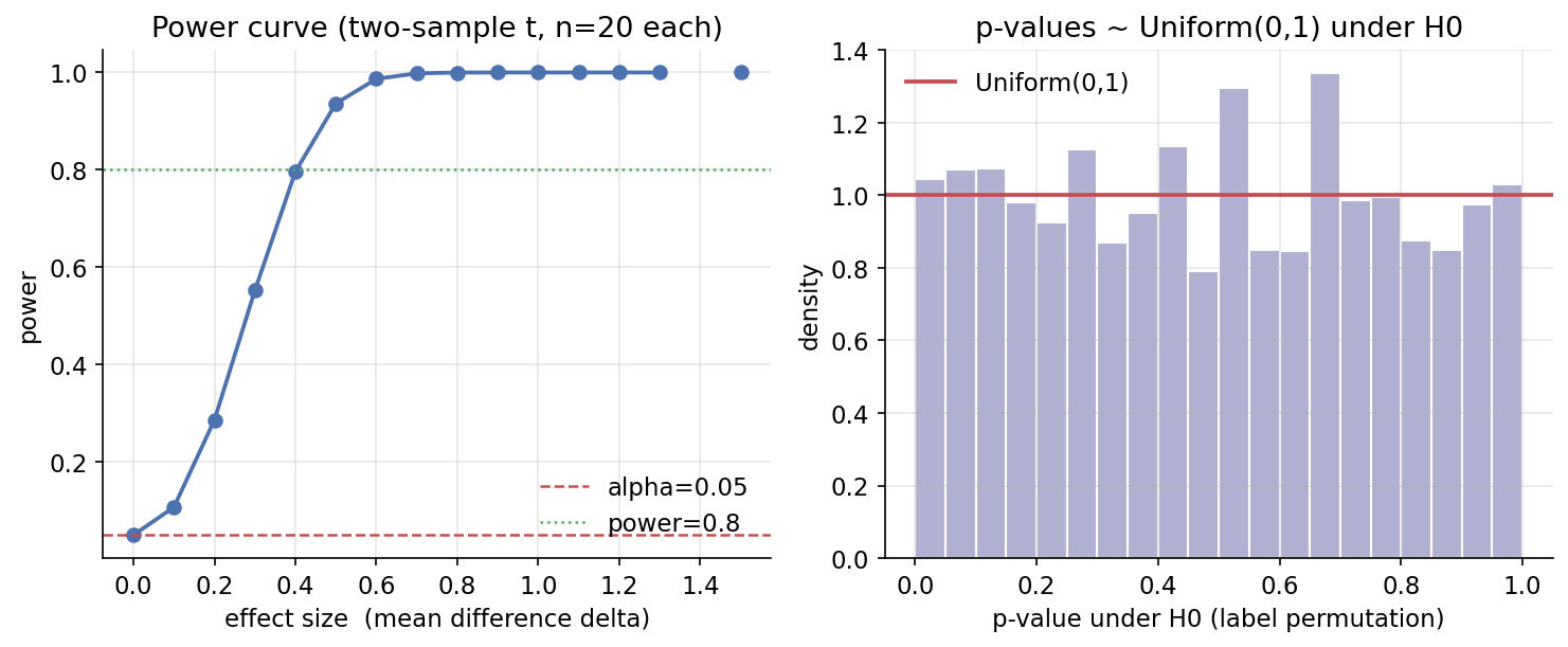
চিত্র: দুই panel — power বনাম effect size (α ও \(0.8\) রেখা সহ), এবং \(H_0\)-এর অধীনে p-value-এর histogram (সমতল \(\approx\) Uniform)।

---

4.8 — Likelihood-ratio · Wald · score tests (একটি proportion)

ধারণা। একই \(H_0\) পরীক্ষার তিনটি asymptotically-সমতুল্য উপায়: Wald (\(\hat p\)-এ estimated info), score/LM (\(p_0\)-এ info), likelihood-ratio (LRT) (\(-2\log\Lambda\))। breast_cancer-এ malignant হার \(p\) পরীক্ষা \(H_0:p=p_0\)-এর বিরুদ্ধে; তিন statistic-ই \(\chi^2_1\)-এর দিকে যায় এবং \(n\) বাড়লে একে অপরের সাথে মিলে যায়।

Scratch-এর মূল ধারণা। malignant indicator (\(p_0=0.40\))-এ Wald \(=(\hat p-p_0)^2/[\hat p(1-\hat p)/n]\), score \(=(\hat p-p_0)^2/[p_0(1-p_0)/n]\), LRT \(=2[\ell(\hat p)-\ell(p_0)]\); তারপর subsample করে বিভিন্ন \(n\)-এ তিনটির ব্যবধান দেখা।

Demonstrated result (প্রমাণ)। \(\hat p=0.372583,\ n=569,\ p_0=0.40\): Wald \(=1.829605\), Score \(=1.782074\), LRT \(=1.796760\) — খুব কাছাকাছি। \(\chi^2_1\) p-value যথাক্রমে \(0.1762,\ 0.1819,\ 0.1801\) (কেউই \(H_0\) নাকচ করে না)। statsmodels-এর score-variance \(z^2=1.782074\) scratch score-এর সাথে হুবহু (True)। \(n\) বাড়লে সর্বোচ্চ pairwise gap statistic-এর তুলনায় সঙ্কুচিত (\(n{=}30\!:0.179\) থেকে বৃহৎ-\(n\)-এ relative-ভাবে অনেক ছোট) — asymptotic equivalence।

\[W=1.830,\quad S=1.782,\quad \text{LRT}=1.797\ \ (\text{সবই}\ \chi^2_1),\qquad W,S,\text{LRT}\ \text{মিলে যায়}\ n\to\infty.\]

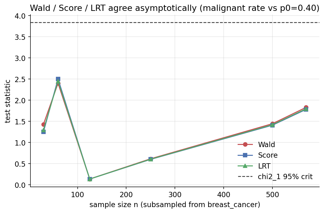
চিত্র: subsample-size \(n\)-এর ফাংশনে Wald/Score/LRT (এবং \(\chi^2_1\) critical) — বড় \(n\)-এ একত্রিত।

---

4.9 — Bootstrap · jackknife · permutation (mean-এর পার্থক্য)

ধারণা। তিনটি resampling হাতিয়ার একসাথে: bootstrap (with-replacement resample করে CI), jackknife (একটা করে datum বাদ দিয়ে bias/SE আন্দাজ), permutation test (\(H_0\)-এর অধীনে label এলোমেলো করে exact p-value)। target: iris virginica ও versicolor-এর petal length-এর mean-এর পার্থক্য।

Scratch-এর মূল ধারণা। observed \(\theta=\bar a-\bar b\); \(B=20{,}000\) bootstrap resample থেকে percentile CI ও SE; pooled sample-এ leave-one-out jackknife থেকে bias ও SE; \(20{,}000\) label-permutation থেকে two-sided p।

Demonstrated result (প্রমাণ)। virginica petal length mean \(=5.5520\), versicolor \(=4.2600\) (\(n=50\) each), observed diff \(\theta=1.292000\)। bootstrap \(95\%\) CI \(=[1.0940,1.4940]\) (SE \(=0.1015\)) — \(0\) বাদ দেয়; scipy bootstrap SE-ও \(0.1015\) (True)। jackknife bias \(=0.0\), jackknife SE \(=0.1030\) (difference-in-means unbiased)। permutation p \(=5\times10^{-5}\) (scipy \(=1\times10^{-4}\), দুটোই নগণ্য)। permutation null centered at \(+0.0030\approx 0\) (sd \(0.1638\)); observed \(\theta\) null থেকে \(7.9\) SD দূরে — অত্যন্ত significant।

\[\theta=1.292,\quad \text{boot CI}=[1.094,\ 1.494]\ (\not\ni 0),\quad p_{\text{perm}}=5\times10^{-5},\quad \text{jackknife bias}=0.\]

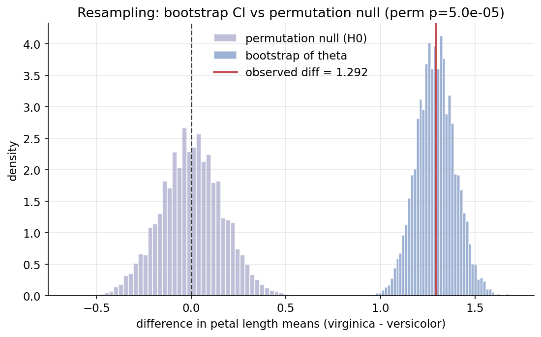
চিত্র: permutation null (ধূসর, \(0\)-কেন্দ্রিক) ও bootstrap distribution (নীল, \(\theta\)-কেন্দ্রিক); observed diff অনেক ডানে — দুটো বণ্টন প্রায় বিচ্ছিন্ন।

---

4.10 — Bayesian inference (Beta–Binomial · Normal–Normal)

ধারণা। Bayesian পদ্ধতি parameter সম্পর্কে posterior distribution দেয়: posterior \(\propto\) likelihood \(\times\) prior। Beta–Binomial: prior \(\text{Beta}(\alpha,\beta)\)-এ \(k\)/\(n\) সাফল্য দিলে posterior \(\text{Beta}(\alpha+k,\ \beta+n-k)\)। Normal–Normal: জানা variance-এ posterior mean হলো prior ও data-এর precision-weighted গড়। এদের \(95\%\) credible interval frequentist CI-এর সাথে তুলনা।

Scratch-এর মূল ধারণা। breast_cancer malignant proportion-এ Beta(1,1) prior → posterior Beta\((1+k,1+n-k)\); iris sepal width-এ Normal prior \(N(3.0,0.5^2)\) ও known \(\sigma\) → precision-weighted posterior; scipy দিয়ে credible interval।

Demonstrated result (প্রমাণ)। Beta–Binomial: \(n=569,\ k=212\) → posterior Beta(213, 358), mean \(=0.373030\), sd \(=0.020221\), \(95\%\) credible \(=[0.3338,0.4131]\)। frequentist Wald CI \(=[0.3329,0.4123]\) (\(\hat p=0.3726\)) — uniform prior ও বড় \(n\)-এ প্রায় অভিন্ন। Normal–Normal: \(\bar x=3.0573,\ \sigma=0.4359,\ n=150\) → posterior mean \(=3.057044\), sd \(=0.035499\), credible \(=[2.9875,3.1266]\) বনাম frequentist t-CI \(=[2.9870,3.1277]\) — আবারও প্রায় মিলে যায়। scipy-র Beta mean/var scratch-এর সাথে হুবহু (True)।

\[\text{posterior}=\text{Beta}(213,358),\quad \text{credible}=[0.334,0.413]\ \approx\ \text{Wald CI}=[0.333,0.412].\]

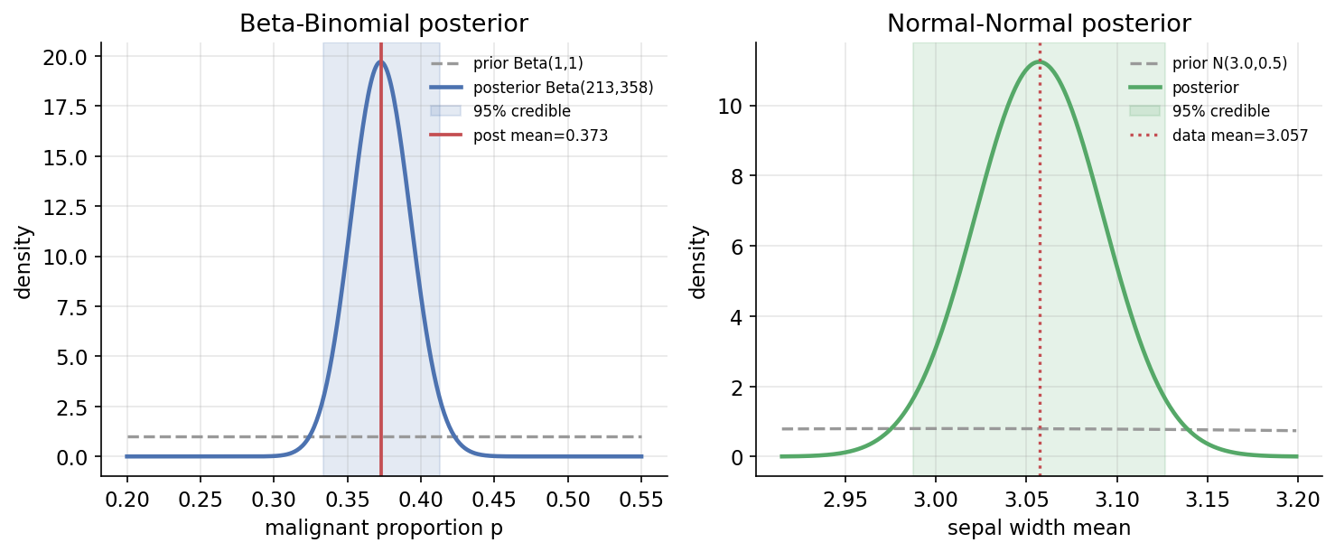
চিত্র: দুই panel — Beta(1,1) prior থেকে সঙ্কুচিত Beta posterior (\(95\%\) credible ছায়া সহ); এবং Normal–Normal prior→posterior।

---

সারসংক্ষেপ (Part IV)

Demo	মূল real ফলাফল
4.1 sampling dist.	median SE \(=0.1596\); sd/SE \(=22.1\times\)
4.2 method of moments	\(k=3.682,\ \theta=0.0248\); \(k\theta,k\theta^2\) হুবহু sample moment; KS \(p=0.50\)
4.3 MLE	\(\hat\mu=5.8433,\ \hat\sigma^2=0.6811\); score at MLE \(\approx 0\)
4.4 estimator props	ddof\(=1\) unbiased; MSE \(\to 0\) (consistency)
4.5 Fisher/CRLB	\(I(\mu)=8.076\); Var/CRLB \(=1.00\) (efficient)
4.6 confidence int.	t-CI \(=[4.906,5.106]\); coverage \(=95.24\%\)
4.7 hypothesis test	\(t=-10.52,\ p\approx 9\times10^{-18}\); power\((\delta{=}0.5)=0.94\); \(p\mid H_0\sim\) Uniform
4.8 LRT/Wald/score	\(W=1.830,\ S=1.782,\ \text{LRT}=1.797\) (মিলে যায়)
4.9 resampling	\(\theta=1.292\); boot CI \(=[1.094,1.494]\); perm \(p=5\times10^{-5}\)
4.10 Bayesian	posterior Beta(213,358); credible \(\approx\) frequentist CI