Part III — convergence (অভিসারণ) ও process · Integrative Demos
Part III পরিসংখ্যানের সেই স্তম্ভগুলো ধরে যেখানে "একটা random পরিমাণ কীভাবে থিতু হয়" আর "সময়ের সাথে এলোমেলো ব্যাপার কীভাবে গড়ায়" — তা গণিত-কঠোরভাবে বোঝা যায়: probability inequalities, modes of convergence, Law of Large Numbers, Central Limit Theorem ও delta method, random processes (Poisson process, AR(1)), এবং Markov chains ও MCMC। এই module-এ প্রতিটি ধারণা চারভাবে দেখানো — (b) scratch (শুধু numpy), (c) library check, (d) demonstrate/"prove" (ছাপা real সংখ্যা), (e) visualization — সবই real open data (iris, sunspots, breast_cancer, co2)-এর উপর, fixed seed 20260619 সহ। নিচের সব সংখ্যা executed notebook (notebooks/03-convergence-processes.ipynb) থেকে সরাসরি নেওয়া।
চালানো:
cd notebooks && python3 -m nbconvert --to notebook --execute --inplace 03-convergence-processes.ipynb --ExecutePreprocessor.timeout=900
3.1 — Probability inequalities (Markov · Chebyshev · Hoeffding)
ধারণা। একটা bounded feature-এর sample mean \(\bar X_n\) তার population mean \(\mu\) থেকে কমপক্ষে \(t\) সরে যাওয়ার সম্ভাবনা \(P(\lvert \bar X_n-\mu\rvert \ge t)\) — এই tail-কে না জেনেই তিনটি inequality উপর থেকে বাঁধে। Markov (\(Z=(\bar X_n-\mu)^2\ge 0\)-এ প্রয়োগ) দেয় \(P(\lvert \bar X_n-\mu\rvert\ge t)\le (\sigma^2/n)/t^2\), যা এখানে Chebyshev \(\dfrac{\sigma^2}{n\,t^2}\)-এর সমান। Hoeffding (feature \([a,b]\)-তে bounded হলে) দেয় \(2\exp\!\big(-2 n t^2/(b-a)^2\big)\) — এটি variance জানে না, শুধু range জানে; তাই এর শক্তি \(n\)-এ exponential decay।
Scratch-এর মূল ধারণা। breast_cancer-এর mean radius min–max scale করে \([0,1]\)-এ আনা হয়। population \(\mu,\sigma\) পুরো column থেকে। তারপর \(B=80{,}000\) বার \(n=20\)-size bootstrap resample করে empirical tail \(\hat P(\lvert\bar X-\mu\rvert\ge t)\) গোনা হয়, আর তিনটি bound formula-তে বসিয়ে তুলনা করা হয়।
Demonstrated result (প্রমাণ)। feature-এ \(\mu=0.338222,\ \sigma=0.166641\) (\(N=569\))। \(t=0.10\)-তে empirical tail \(=0.007587\), আর তিন bound: Markov \(=\) Chebyshev \(=0.138846\), Hoeffding \(=1.340640\)। তিনটিই ধরে রাখে (\(\text{empirical}\le\text{bound}\)):
তুলনামূলক টাইটনেস: Chebyshev empirical-এর \(18.3\times\), Hoeffding \(176.7\times\) — অর্থাৎ এই low-variance feature-এ Chebyshev অনেক টাইট, কারণ সে প্রকৃত variance (\(\sigma^2=0.0278\)) ব্যবহার করে, আর Hoeffding শুধু worst-case range-variance \((b-a)^2/4=0.25\) ধরে। Hoeffding-এর আসল সুবিধা হলো \(n\) বাড়লে exponential হারে কমা। একটা sanity: normal-approx (CLT) tail \(2\lbrack 1-\Phi(z)\rbrack=0.007281\) (\(z=2.6837\)) — empirical-এর খুব কাছে।
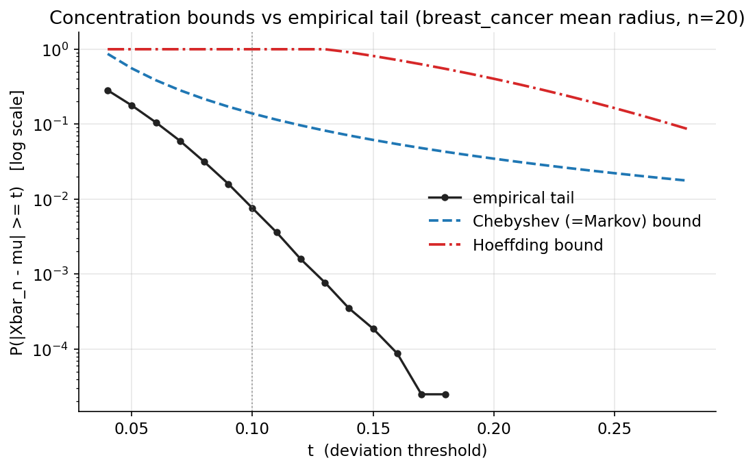
চিত্র: breast_cancer mean radius-এ (\(n=20\)) empirical tail বনাম Chebyshev ও Hoeffding bound, \(t\)-এর ফাংশন হিসেবে (log-scale); দুটি bound-ই empirical curve-এর উপরে থাকে।
3.2 — Types of convergence (in probability বনাম almost-sure)
ধারণা। \(Y_n\xrightarrow{P}c\) মানে প্রতি \(\varepsilon>0\)-এ \(P(\lvert Y_n-c\rvert>\varepsilon)\to 0\); \(Y_n\xrightarrow{a.s.}c\) মানে \(P(\lim_n Y_n=c)=1\)। almost-sure শক্তিশালী: a.s. \(\Rightarrow\) in-prob, কিন্তু উল্টোটা নয়। ক্লাসিক পার্থক্য typewriter sequence — block-এর ভিতরে একটাই "\(1\)" ঘুরে বেড়ায় (block length \(L=1,2,3,\dots\)); \(P(Y_n=1)\sim 1/L\to 0\) (in prob) হলেও প্রতিটি path অসীমবার \(1\) ছোঁয়, তাই a.s. converge করে না। বিপরীতে iris feature-এর running mean সত্যিই a.s. থিতু হয়।
Scratch-এর মূল ধারণা। iris petal length-এর resample-stream-এর running mean (cumsum/arange) ও running max (np.maximum.accumulate); সঙ্গে হাতে বানানো typewriter indicator ও তার block-density \(1/L\)।
Demonstrated result (প্রমাণ)। petal length \(\mu=3.758\)। running mean \(n=100\)-এ \(3.701\), \(n=1500\)-এ \(3.798\) (\(\lvert\cdot-\mu\rvert=0.040\)) — মানে থিতু। running max \(n=1500\)-এ \(6.900\) (feature-এর সর্বোচ্চ) — কখনো \(\mu\)-তে থিতু হয় না, একঘেয়ে বাড়ে। almost-sure signature: \(\sup_{m\ge k}\lvert \text{mean}_m-\mu\rvert\) সঙ্কুচিত হয় — \(k=100\!:0.141,\ k=500\!:0.058,\ k=1000\!:0.049\)। typewriter: \(1500\) term-এ মোট \(744\)টি "\(1\)"; \(P(Y_n=1)\) যায় \(1.0\to 0.25\ (n{=}10)\to 0.018\ (n{=}1500)\), অর্থাৎ \(\xrightarrow{P}0\); অথচ \(n=1000\)-এর পরেও \(250\)টি "\(1\)" আছে (\(>0\) চিরকাল) — তাই almost-sure নয়।
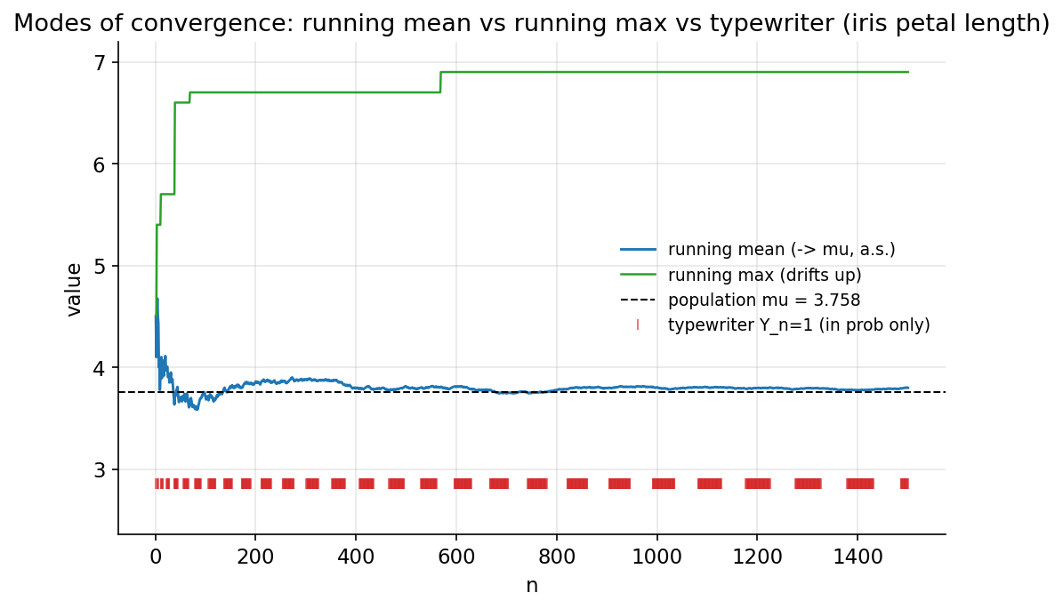
চিত্র: running mean (\(\to\mu\), a.s.), running max (উপরে drift করে), এবং typewriter spike (শুধু in-probability) — iris petal length-এ।
3.3 — Law of Large Numbers (running mean → μ)
ধারণা। LLN বলে iid draw-এর running mean \(\bar X_n\) population mean \(\mu\)-তে যায়; CLT থেকে তার ওঠানামা \(\pm\sigma/\sqrt n\) হারে সঙ্কুচিত। তাই একটা \(\mu\pm\sigma/\sqrt n\) envelope আঁকলে দেখা যায় path-গুলো তার ভিতরে ঢুকে থিতু হচ্ছে।
Scratch-এর মূল ধারণা। iris petal length বারবার (without replacement) shuffle করে \(12\)টি independent running-mean path; theoretical band \(\sigma/\sqrt n\); আর প্রতিটি \(n\)-এ path-দের empirical sd বনাম \(\sigma/\sqrt n\)।
Demonstrated result (প্রমাণ)। \(\mu=3.758,\ \sigma=1.759404\) (\(N=150\))। band সঙ্কুচিত হয়: \(n{=}1\!:1.759,\ n{=}30\!:0.321,\ n{=}150\!:0.144\)। path-বিন্দুর \(99.56\%\) থাকে \(\mu\pm 2\sigma/\sqrt n\)-এর ভিতরে। spread \(\sigma/\sqrt n\)-কে অনুসরণ করে: \(n{=}5\)-এ empirical sd \(0.794\) বনাম theory \(0.787\) (ratio \(1.01\)), \(n{=}20\!:0.282/0.393,\ n{=}50\!:0.176/0.249\)। যেহেতু shuffle সম্পূর্ণ permutation, \(n{=}N{=}150\)-এ প্রতিটি path ঠিক \(\mu\)-তে মেলে (finite-population সীমা; empirical sd \(=0\)) — LLN-এর একেবারে নির্ভুল রূপ।
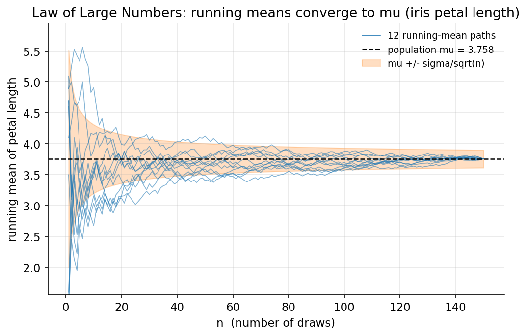
চিত্র: \(12\)টি running-mean path \(\mu\)-তে অভিসারী, সঙ্কুচিত \(\mu\pm\sigma/\sqrt n\) band সহ (iris petal length)।
3.4 — CLT & delta method
ধারণা। যত skewed feature হোক, standardized sample mean \(Z_n=\sqrt n\,(\bar X_n-\mu)/\sigma\xrightarrow{d}N(0,1)\) (CLT)। আর কোনো smooth \(g\)-এর জন্য delta method দেয় \(\operatorname{Var}\!\big(g(\bar X_n)\big)\approx \big(g'(\mu)\big)^2\sigma^2/n\); এখানে \(g=\log\), তাই \(g'(\mu)=1/\mu\)।
Scratch-এর মূল ধারণা। sunspots SUNACTIVITY (\(>0\)) থেকে \(\mu,\sigma\); বাড়তে থাকা \(n\)-এ bootstrap sample mean থেকে \(Z_n\) বানিয়ে histogram ও standard-normal overlay; আর \(\operatorname{Var}(\log\bar X_n)\)-কে \((1/\mu)^2\sigma^2/n\)-এর সঙ্গে তুলনা।
Demonstrated result (প্রমাণ)। feature: \(N=306,\ \mu=50.2399,\ \sigma=40.2815\), skew \(=0.9854\) (ডান দিকে ভারী)। CLT symmetrize করে: skew যায় \(0.9854\to 0.250\ (n{=}20)\to 0.114\ (n{=}60)\to 0.105\); \(n{=}60\)-এ \(Z_n\) mean \(-0.0014\), sd \(1.0079\), আর \(\mathrm{KS}(Z_n,N(0,1))=0.0091\) (খুব ছোট)।
delta method (\(g=\log,\ n=40\)): empirical \(\operatorname{Var}(\log\bar X_n)=1.638570\times10^{-2}\) বনাম predicted \((1/\mu)^2\sigma^2/n=1.607145\times10^{-2}\) — ratio \(=1.0196\) (প্রায় \(1\), formula নিশ্চিত)।
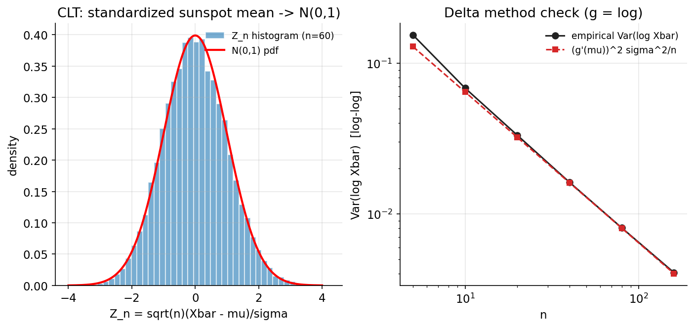
চিত্র (২ প্যানেল): (বাঁ) \(n{=}60\)-এ \(Z_n\)-এর histogram \(N(0,1)\) pdf-এর সাথে মিলছে; (ডান) \(\operatorname{Var}(\log\bar X_n)\) empirical বনাম delta-method prediction, \(n\)-এর log–log-এ প্রায় মিলে যাওয়া রেখা।
3.5 — Random processes (Poisson process · AR(1) on co2)
ধারণা। rate \(\lambda\)-এর homogeneous Poisson process-এ unit-window count \(\sim\text{Poisson}(\lambda)\) ও interarrival time \(\sim\text{Exponential}(\lambda)\)। আর AR(1) \(r_t=\phi\,r_{t-1}+\varepsilon_t,\ \varepsilon_t\sim N(0,\sigma_\varepsilon^2)\) হলো এক সরল Gaussian process যা autocorrelated noise মডেল করে।
Scratch-এর মূল ধারণা। exponential gap (\(\text{Exp}(1/\lambda)\)) যোগ করে event-time; unit-bin-এ count; আর co2 থেকে quadratic-in-time trend বাদ দিয়ে residual, তার উপর no-intercept OLS-এ \(\phi=\sum r_{t-1}r_t/\sum r_{t-1}^2\) ও residual sd থেকে \(\sigma_\varepsilon\)।
Demonstrated result (প্রমাণ)। Poisson (\(\lambda=3,\ T=50\)): observed events \(=157\) (expected \(\lambda T=150\)); unit-bin count mean \(=3.140\), var \(=2.898\) (Poisson-এ mean \(\approx\) var \(\approx\lambda\), dispersion index \(0.923\)); mean interarrival \(=0.3179\) (theory \(1/\lambda=0.3333\)); \(\mathrm{KS}(\text{gaps},\text{Exp})=0.0930\)।
AR(1) on co2 residual (\(n=2225\)): \(\phi=0.973743\), \(\sigma_\varepsilon=0.499128\); scratch \(\phi\) scipy linregress slope-এর সঙ্গে হুবহু মিলেছে, আর lag-1 autocorrelation \(=0.973836\) (\(\approx\phi\), \(1\)-এর কাছাকাছি — শক্তিশালী স্মৃতি)। simulated AR(1) path-এর lag-1 autocorr \(0.9695\) আসল residual-এর \(0.9738\)-এর কাছাকাছি।
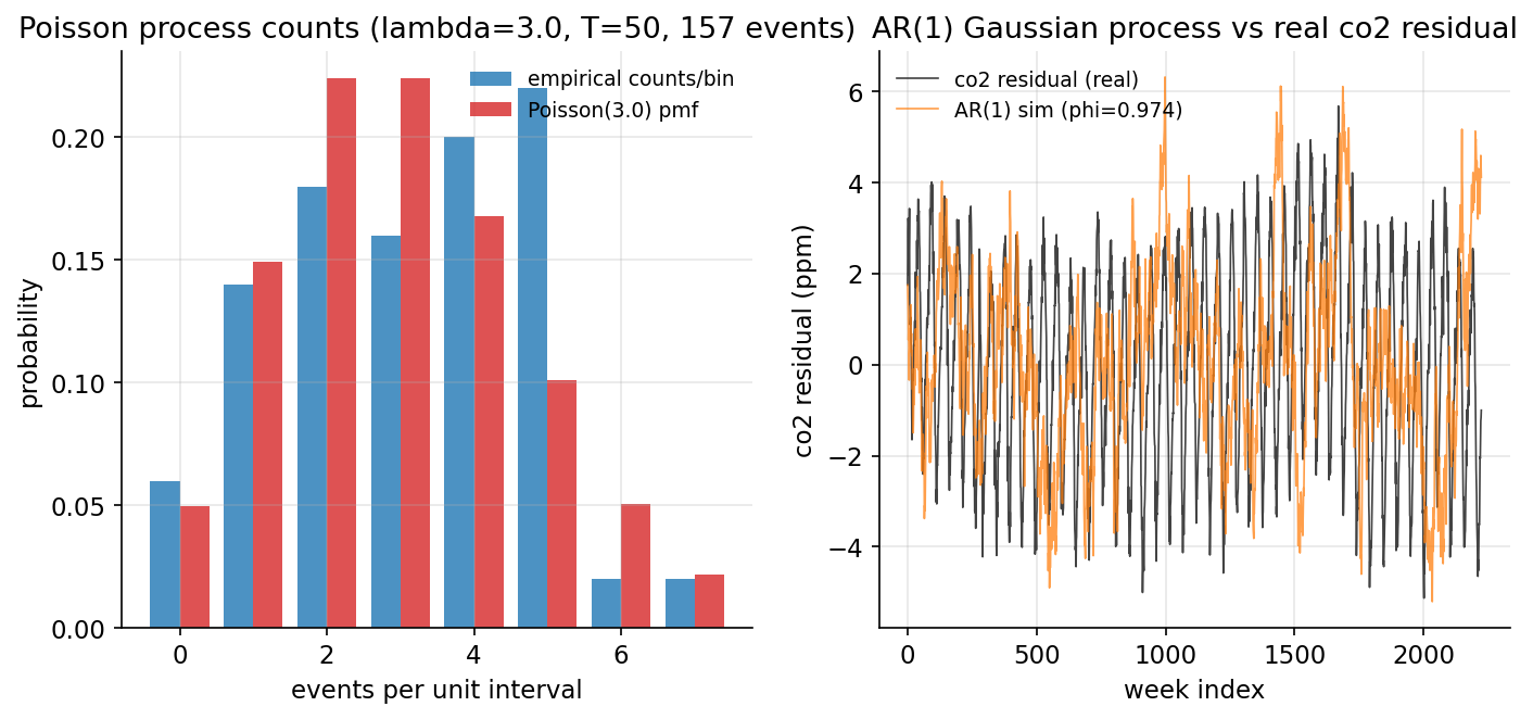
চিত্র (২ প্যানেল): (বাঁ) Poisson process-এর unit-bin count empirical বনাম \(\text{Poisson}(3)\) pmf; (ডান) fitted AR(1) simulated path বনাম আসল co2 de-trended residual।
3.6 — Markov chains & MCMC
ধারণা। finite-state Markov chain-এর ভবিষ্যৎ শুধু বর্তমান state-এর উপর নির্ভর করে। stationary distribution \(\pi\) হলো \(\pi P=\pi\) (eigenvalue \(1\)-এর left eigenvector); \(P^n\)-এর row-গুলো \(\pi\)-তে মিলিত হয়। Metropolis–Hastings (MCMC) কোনো (unnormalized) target \(p\) থেকে sample টানে: proposal \(x'=x+\text{Normal}(0,s)\), accept with prob \(\min\!\big(1,\ p(x')/p(x)\big)\)।
Scratch-এর মূল ধারণা। co2 weekly change \(\Delta\)-কে \(\lbrace\text{down},\text{flat},\text{up}\rbrace\)-এ ভাগ (threshold \(0.1\) ppm); consecutive-pair count থেকে row-normalize করে \(P\); eig(P.T) থেকে \(\pi\); matrix_power দিয়ে \(P^n\); আর একটা bimodal target-এ MH sampler (\(60{,}000\) step, burn-in \(5000\))।
Demonstrated result (প্রমাণ)। state count \(\lbrace\text{down},\text{flat},\text{up}\rbrace=\lbrace840,312,1072\rbrace\)। transition matrix
\(\pi\) একটি বৈধ probability vector এবং \(\pi P=\pi\) যাচাই হয়েছে। \(P^n\)-এর row-0 দ্রুত \(\pi\)-তে মিলিত: \(\lVert P^n\text{row}_0-\pi\rVert_1\) যায় \(2.04\times10^{-1}\ (n{=}1)\to 3.56\times10^{-2}\ (n{=}2)\to 1.85\times10^{-4}\ (n{=}5)\to 9.99\times10^{-16}\ (n{=}20)\)। MH (\(s=1.5\)): acceptance rate \(0.5516\), sample mean \(0.0366\) বনাম numeric target mean \(\approx 0.0000\); histogram-vs-target mean \(\lvert\text{density diff}\rvert=0.0029\) (খুব ছোট, ভালো মিল)।
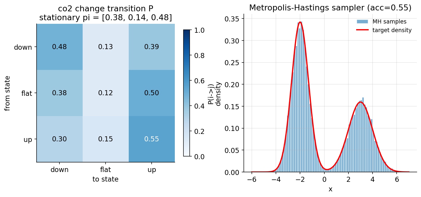
চিত্র (২ প্যানেল): (বাঁ) co2 change-এর transition matrix \(P\)-এর heatmap, নিচে stationary \(\pi\); (ডান) MH-এর sampled histogram bimodal target density-র সাথে মিলছে।
সারাংশ (numbers-at-a-glance)। 3.1 empirical tail \(0.007587\le\) Chebyshev \(0.1388\le\) Hoeffding \(1.3406\); 3.2 running mean \(\to 3.758\), typewriter \(P(Y_n{=}1){\to}0.018\) কিন্তু a.s. নয়; 3.3 band \(1.759{\to}0.144\), spread ratio \(\approx 1\); 3.4 skew \(0.985{\to}0.105\), KS \(0.0091\), delta ratio \(1.0196\); 3.5 Poisson mean/var \(3.14/2.90\), AR(1) \(\phi=0.9737\); 3.6 \(\pi=(0.378,0.140,0.482)\), \(\lVert P^{20}\text{row}-\pi\rVert_1\approx 10^{-15}\), MH acc \(0.55\)।