Part VII — measure-তাত্ত্বিক (মেজার) সম্ভাব্যতা · Integrative Demos
Part VII পরিসংখ্যানের সবচেয়ে বিমূর্ত ভিত্তি ধরে — measure theory — এবং দেখায় সেটি আসলে real data-র সবচেয়ে গভীর নিয়মের ভাষা: কেন Riemann integral যথেষ্ট নয়, σ-algebra ও measure কী, measurable map ও pushforward, Lebesgue integral = averaging, \(L^p\)/Hilbert/Radon–Nikodym, SLLN, conditional expectation = ANOVA, martingale ও তার convergence, এবং শেষে characteristic function দিয়ে CLT — পুরো ascent-এর চূড়া। এই module-এ প্রতিটি ধারণা চারভাবে দেখানো — (b) scratch (শুধু numpy), (c) library/analytic check, (d) demonstrate/"prove" (ছাপা real সংখ্যা), (e) visualization (একটি করে figure, savefig) — বেশিরভাগই real open data (iris, breast_cancer, co2)-এর উপর, আর যেখানে measure theory দাবি করে সেখানে analytic object-এ; fixed seed 20260619 সহ। নিচের সব সংখ্যা executed notebook (notebooks/07-measure-theoretic.ipynb) থেকে সরাসরি নেওয়া।
চালানো:
cd notebooks && python3 -m nbconvert --to notebook --execute --inplace 07-measure-theoretic.ipynb --ExecutePreprocessor.timeout=1200
7.1 — Why measure theory (Dirichlet · measure-zero cover · Cantor set)
ধারণা। Riemann integral-এর তিনটি crack (ফাটল) measure theory-র জন্ম দেয়। Dirichlet function \(\mathbf 1_{\mathbb Q}\) প্রতিটি sub-interval-এ rational ও irrational দুইই ধরে, তাই Riemann upper sum \(=1\), lower sum \(=0\) — কখনো মেলে না, ফাংশনটি Riemann-অসংগত; অথচ Lebesgue-এ \(\int_0^1\mathbf 1_{\mathbb Q}\,d\lambda=\lambda(\mathbb Q\cap[0,1])=0\)। Measure zero: \(\mathbb Q\cap[0,1]\) countable, তাই \(q_k\)-কে দৈর্ঘ্য \(\varepsilon/2^k\)-এর interval দিয়ে ঢাকলে মোট \(\le\sum_k\varepsilon/2^k=\varepsilon\to 0\)। Cantor set \(C\): বারবার মাঝের \(1/3\) ফেললে \(\lambda(C)=\lim(2/3)^n=0\), তবু uncountable (dimension \(\log 2/\log 3\))।
Scratch-এর মূল ধারণা। যেকোনো partition-এ Dirichlet-এর প্রতি cell-এ \(\sup=1,\ \inf=0\) ধরে upper/lower sum; rational grid \(k/1000\)-এ evaluate করলে সব \(1\), irrational-ঘেঁষা বিন্দুতে সব \(0\)। তারপর \(\varepsilon\)-cover-এর মোট দৈর্ঘ্য \(\sum\varepsilon/2^k\) ছাপা এবং Cantor-এর surviving interval-দৈর্ঘ্য \((2/3)^n\)।
Demonstrated result (প্রমাণ)। Dirichlet: upper sum \(=1.0000\), lower sum \(=0.0000\), gap \(=1.0000\) (কখনো \(\to 0\) নয়) — Riemann-অসংগত; Lebesgue value \(=0.0000\) (rational-দের মাপ)। \(\varepsilon\)-cover: \(\varepsilon=1,0.1,0.01,0.001\)-এ মোট দৈর্ঘ্য যথাক্রমে \(1.0,0.1,0.01,0.001\) — যত ছোট \(\varepsilon\) চাই তত ছোট, তাই \(\lambda(\mathbb Q\cap[0,1])=0\)। Cantor: \(k=20\) ধাপে দৈর্ঘ্য \((2/3)^{20}=3.007\times10^{-4}\to 0\), dimension \(\log 2/\log 3=0.630930\) (uncountable dust)।
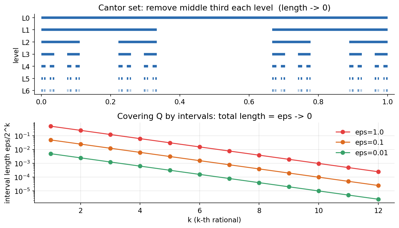
চিত্র: Cantor set-এর ধাপে-ধাপে নির্মাণ (দৈর্ঘ্য \(\to 0\)) এবং rational-দের \(\varepsilon/2^k\)-interval দিয়ে ঢাকা (মোট দৈর্ঘ্য \(=\varepsilon\to 0\))।
7.2 — σ-algebra ও measure (empirical measure \(\mu_n\))
ধারণা। একটা σ-algebra \(\mathcal F\) complement ও countable union-এ বন্ধ; তার উপর measure \(\mu\) দেয় \(\mu(\varnothing)=0\) ও disjoint set-এ countable additivity। সবচেয়ে বাস্তব measure হলো empirical measure \(\mu_n(A)=\#\{x_i\in A\}/n\) — একটি genuine probability measure, আর Glivenko–Cantelli-র ভাবনায় \(n\) বাড়লে \(\mu_n(A)\to P(A)\)।
Scratch-এর মূল ধারণা। iris petal length-কে \(6\)টি disjoint bin-এ ভাগ; প্রতিটি bin-এ \(\mu_n=\text{proportion}\) হাতে গোনা; একটা fixed bin-এ resample-size \(n\) বাড়িয়ে \(\mu_n(A)\)-কে full-sample proportion-এর দিকে যেতে দেখা; সব disjoint bin-এর measure যোগ করে countable additivity (\(=1\)) যাচাই।
Demonstrated result (প্রমাণ)। bin edges \([1.0,1.98,2.97,3.95,4.93,5.92,6.9]\); full-sample bin-measure \([0.333,0,0.073,0.287,0.233,0.073]\), যোগফল \(=1.000000\) (countable additivity)। target bin \(A=[1.0,1.983)\), true \(P(A)=0.33333\); resample \(\mu_n(A)\): \(n{=}10\!:0.200,\ n{=}30\!:0.333,\ n{=}100\!:0.330,\ n{=}1000\!:0.335,\ n{=}5000\!:0.343\) — সত্য মানের চারপাশে থিতু। scratch \(\mu\) == np.histogram proportions (\(\text{True}\)); \(\mu_n(\text{whole support})=1.0\)।
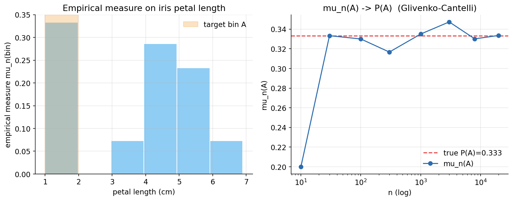
চিত্র: iris petal length-এর empirical measure (histogram, target bin highlighted) এবং \(\mu_n(A)\to P(A)\) যত \(n\) বাড়ে (Glivenko–Cantelli)।
7.3 — Measurable map ও pushforward law \(P_Y=g_\#P_X\)
ধারণা। \(g\) measurable হলে \(Y=g(X)\)-এর আইন pushforward \(P_Y(B)=P_X(g^{-1}(B))\); monotone smooth \(g\)-তে change-of-variables \(f_Y(y)=f_X(g^{-1}(y))\lvert\frac{d}{dy}g^{-1}(y)\rvert\)। সবচেয়ে গুরুত্বপূর্ণ পরিচয় (law of the unconscious statistician): \(\mathbb E[g(X)]=\int g\,dP_X=\frac1n\sum_i g(x_i)\) — \(Y\)-এর নতুন আইন না বের করেও।
Scratch-এর মূল ধারণা। iris petal length \(X\)-এ \(g(x)=x^2\) বসিয়ে \(Y=X^2\)-এর histogram; KDE দিয়ে \(f_X\) estimate করে analytic transform density \(f_Y(y)=f_X(\sqrt y)/(2\sqrt y)\); আর \(\int g\,d\mu_n=\frac1n\sum g(x_i)\) ছাপা।
Demonstrated result (প্রমাণ)। \(X\in[1.00,6.90]\), \(Y=X^2\in[1.00,47.61]\); sample mean of \(Y=\text{mean}(g(x_i))=17.218067\)। \(\int g\,d\mu_n\) (empirical) \(=17.218067\) — exact identity holds: True। KDE-smoothed \(\int g(x)f_X(x)\,dx=16.506453\) (কাছাকাছি; পার্থক্য শুধু KDE bias \(0.712\))। analytic \(\int f_Y\,dy=0.898\) (\(\approx 1\)), \(\int y\,f_Y\,dy=16.51\) — pushforward density-ও একই E[Y]-এর দিকে।
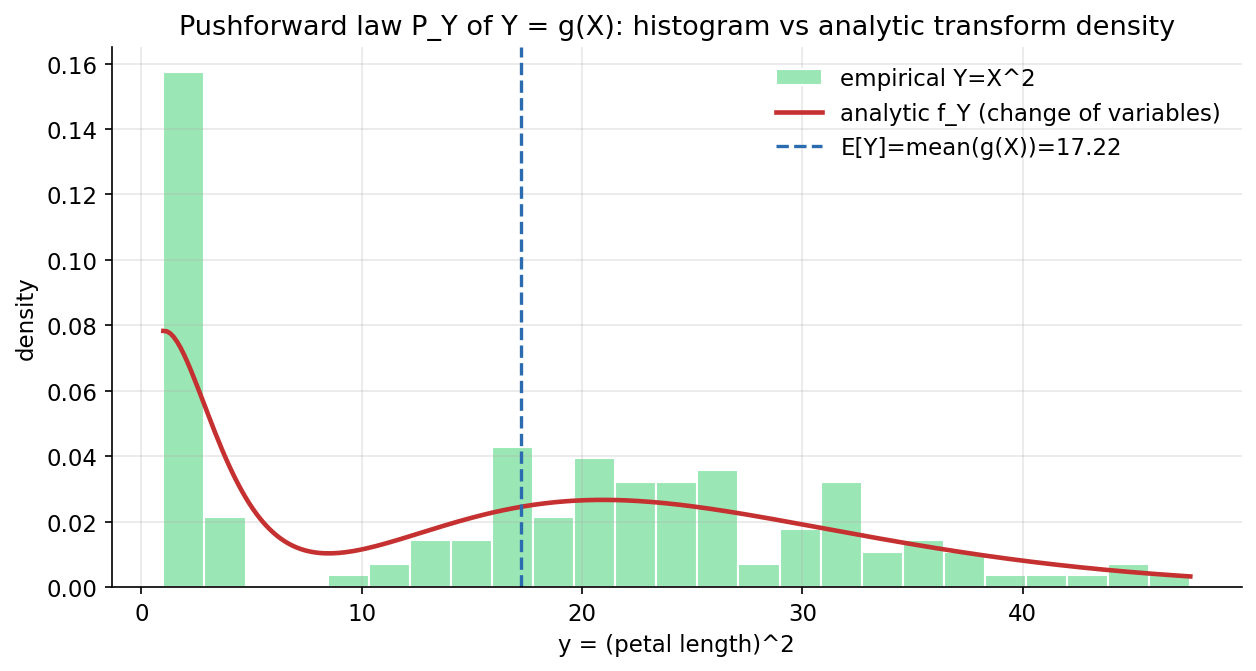
চিত্র: \(Y=X^2\)-এর empirical histogram বনাম analytic change-of-variables density \(f_Y\) (iris petal length); খাড়া রেখা \(\mathbb E[Y]=\text{mean}(g(X))\)।
7.4 — Lebesgue integral = averaging (\(\int f\,d\mu_n\)) ও MCT
ধারণা। empirical measure-এর সাপেক্ষে Lebesgue integral ঠিক sample average: \(\int f\,d\mu_n=\sum_i f(x_i)\mu_n(\{x_i\})=\frac1n\sum_i f(x_i)\) — "integrate w.r.t. \(\mu_n\)" মানে "গড় নাও"। Monotone Convergence Theorem (MCT): \(0\le f_1\le f_2\le\cdots\uparrow f\) হলে \(\int f_n\,d\mu\uparrow\int f\,d\mu\) — limit ও integral বদলানো নিরাপদ।
Scratch-এর মূল ধারণা। breast_cancer 'mean area' (heavy right tail)-এ \(\int f\,d\mu_n=\frac1n\sum f(x_i)\); তারপর truncation \(f_n=\min(f,\text{cap})\)-এর integral cap বাড়ার সাথে monotonically বাড়ে ও পুরো গড়ে থিতু হয়।
Demonstrated result (প্রমাণ)। \(\int f\,d\mu_n\) (scratch) \(=654.889104\) == np.mean \(=654.889104\) (True); mean \(654.89 \gg\) median \(551.10\) (right-skewed, max \(2501\))। MCT staircase (cap : integral, fraction): \(200\!:199.78\ (0.305),\ 600\!:501.97\ (0.767),\ 1000\!:605.09\ (0.924),\ 1500\!:645.64\ (0.986),\ 3000\!:654.89\ (1.000)\) — monotone nondecreasing: True, cap \(\to\) max-এ \(\int f_n\uparrow\int f=654.8891\)।
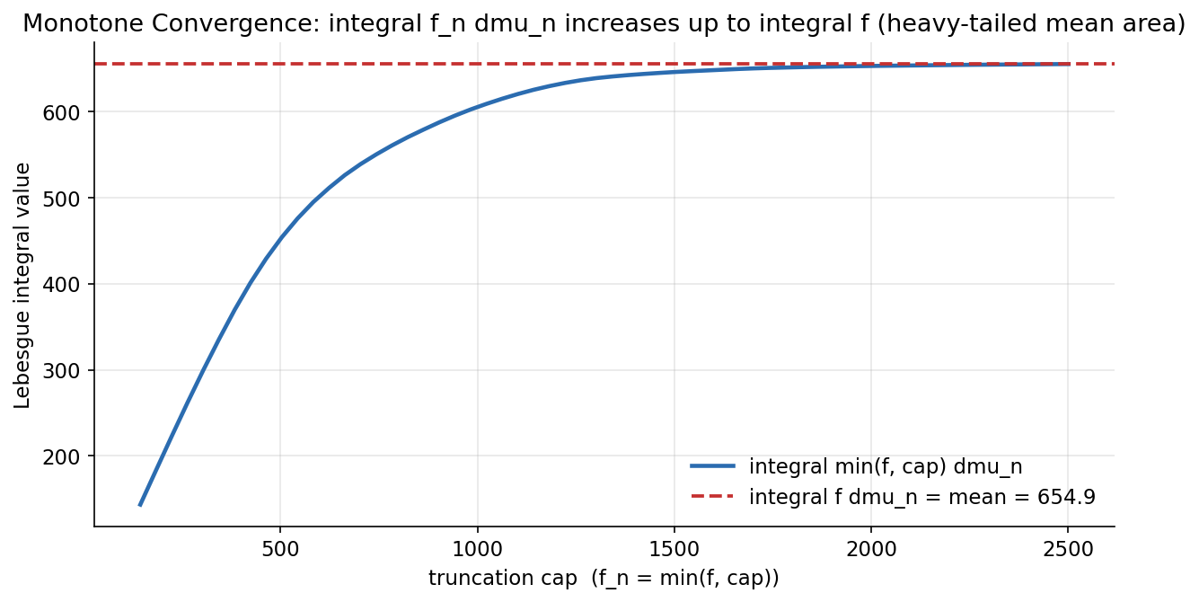
চিত্র: \(\int\min(f,\text{cap})\,d\mu_n\) cap বাড়ার সাথে একঘেয়ে বেড়ে full mean (\(654.9\))-এ থিতু হয় (breast_cancer mean area) — Monotone Convergence Theorem।
7.5 — \(L^p\) / Hilbert space / Radon–Nikodym
ধারণা। তিনটি স্তম্ভ: \(L^p\) norm \(\lVert X\rVert_p=(\frac1n\sum\lvert x_i\rvert^p)^{1/p}\) bounded support-এ \(p\)-তে অ-হ্রাসমান, \(p\to\infty\)-এ \(\lVert X\rVert_\infty=\max\lvert x_i\rvert\) (power-mean inequality)। \(L^2\) = Hilbert space: grouping σ-algebra \(\mathcal G\)-এর orthogonal projection হলো \(\mathbb E[X\mid\mathcal G]=\) group means, যা \(L^2\) error minimize করে। Radon–Nikodym derivative \(\frac{dP}{dQ}\) = দুই subgroup-এর density ratio (likelihood ratio)।
Scratch-এর মূল ধারণা। iris sepal length-এ \(\lVert X\rVert_p\) একটা p-grid-এ; species group means = \(L^2\) projection ও তার error বনাম grand-mean error; breast_cancer-এ malignant বনাম benign-এর KDE density-র অনুপাত \(f_{\text{mal}}/f_{\text{ben}}\)।
Demonstrated result (প্রমাণ)। \(\lVert X\rVert_p\): \(p{=}1\!:5.843,\ p{=}2\!:5.901,\ p{=}10\!:6.338,\ p{=}50\!:7.270\to\lVert X\rVert_\infty=7.900\) (nondecreasing: True)। group means \(\mathbb E[X\mid\text{species}]=\{5.006,5.936,6.588\}\); \(L^2\) error group-mean \(=0.259708\) বনাম grand-mean \(=0.681122\); \(20000\) perturbation-এর মধ্যে সেরা \(=0.259800\) — group means হলো \(L^2\)-optimal (True)। RN ratio malignant/benign: radius \(10\)-এ \(0.053\) (benign-heavy), radius \(20\)-এ \(1.09\times10^{5}\) (malignant-heavy)।
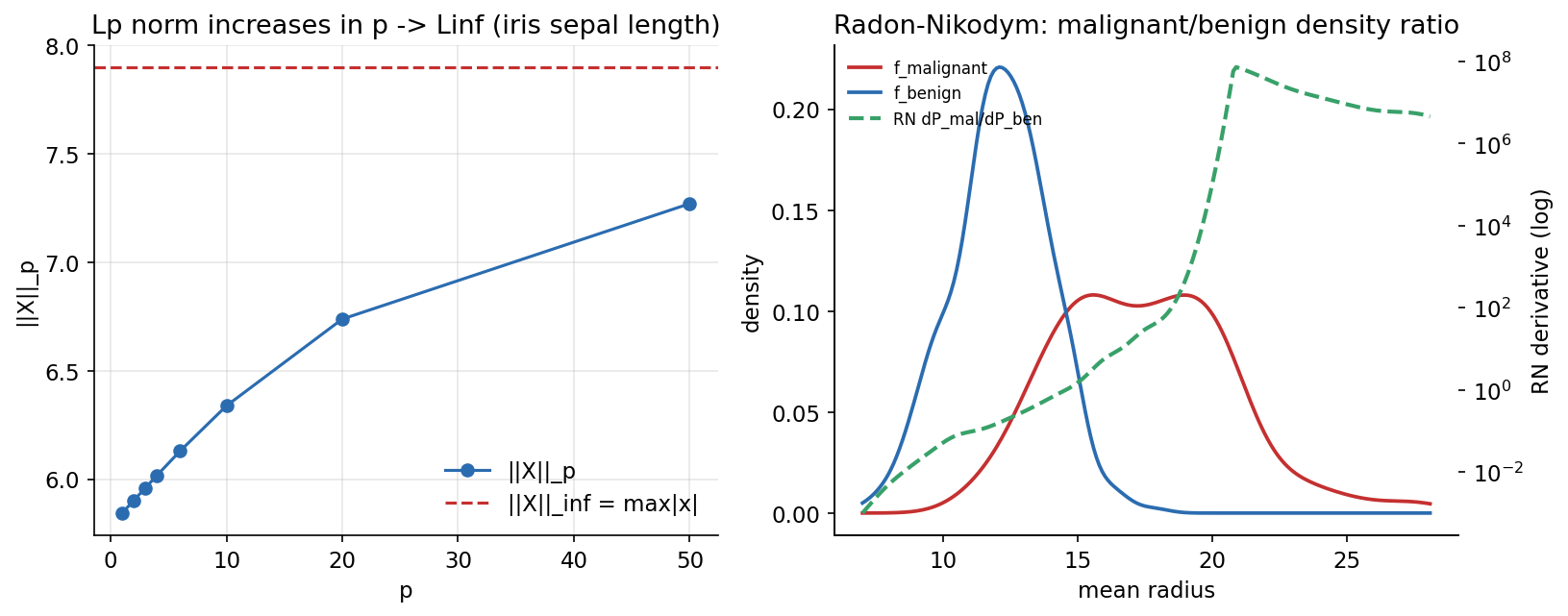
চিত্র: (বামে) \(\lVert X\rVert_p\) \(p\)-তে বেড়ে \(\lVert X\rVert_\infty\)-এ যায়; (ডানে) malignant ও benign density এবং তাদের অনুপাত = Radon–Nikodym derivative (log-scale)।
7.6 — Independence ও Strong Law of Large Numbers (SLLN)
ধারণা। SLLN: iid হলে running mean \(\bar X_n\xrightarrow{a.s.}\mu\) — প্রায় প্রতিটি path probability \(1\)-এ \(\mu\)-তে থিতু। Borel–Cantelli: \(\sum_n P(A_n)<\infty\) হলে \(P(A_n\ \text{i.o.})=0\), তাই rare event শুধু finitely often ঘটে। Independence measure-তাত্ত্বিকভাবে joint law \(=\) product law।
Scratch-এর মূল ধারণা। iris petal length-কে বারবার permute করে \(30\)টি a.s. running-mean path; সব path-এর max deviation থেকে \(\mu\) সঙ্কুচিত; rare event \(\{x>c\}\) (\(c=\) top \(3\%\))-এর সঞ্চিত গণনা; দুই feature-এর correlation ও \(\chi^2\) test।
Demonstrated result (প্রমাণ)। \(\mu=3.758\); সব \(30\) path-এ \(n{=}N\)-এ \(\max\lvert\bar X_N-\mu\rvert=2.22\times10^{-15}\) (full permutation-এ ঠিক \(\mu\))। max deviation (\(n\): value): \(10\!:1.152,\ 30\!:0.595,\ 100\!:0.241,\ 149\!:0.021\) — পুরো ensemble \(\mu\)-তে funnels (a.s.)। Borel–Cantelli: rare threshold \(c=6.353\) (\(P{\approx}0.033\)), মোট rare event \(=5\) (সসীম)। independence: corr(petal L, petal W) \(=0.9629\) (strongly dependent), \(\chi^2=241.26,\ p=4.98\times10^{-51}\) (reject independence); corr(sepal W, petal L) \(=-0.4284\) (weak)।
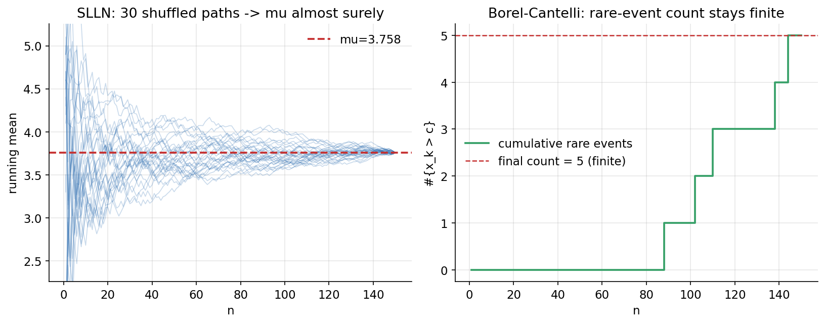
চিত্র: (বামে) \(30\)টি shuffled running-mean path প্রায়-নিশ্চিতভাবে \(\mu=3.758\)-এ অভিসারী; (ডানে) rare-event (\(x>c\))-এর সঞ্চিত গণনা সসীম (\(5\))-এ থেমে থাকে (Borel–Cantelli)।
7.7 — Conditional expectation ও law of total variance = ANOVA
ধারণা। grouping σ-algebra \(\mathcal G=\sigma(\text{species})\)-এর উপর \(\mathbb E[X\mid\mathcal G]=\) group means হলো \(L^2\)-এর best predictor (regression onto grouping)। Law of total variance: \(\operatorname{Var}(X)=\mathbb E[\operatorname{Var}(X\mid\mathcal G)]+\operatorname{Var}(\mathbb E[X\mid\mathcal G])\) — হুবহু within \(+\) between = ANOVA, আর \(R^2=\text{between}/\text{total}\)।
Scratch-এর মূল ধারণা। iris petal length-এ group means = conditional expectation; within \(=\) E[Var(X\mid G)] (weighted group variances), between \(=\) Var(E[X\mid G]); যোগফল total-এর সমান কিনা; tower property \(\mathbb E[\mathbb E[X\mid G]]=\) grand mean।
Demonstrated result (প্রমাণ)। \(\mathbb E[X\mid\text{species}]=\{1.462,4.260,5.552\}\); within \(=0.181484\), between \(=2.914019\); total \(\operatorname{Var}(X)=3.095503\), within\(+\)between \(=3.095503\) — law of total variance holds: True। tower: \(\mathbb E[\mathbb E[X\mid G]]=3.758000=\) grand mean (True)। \(R^2=\text{between}/\text{total}=0.941372\); ANOVA \(F=1180.16,\ p=2.86\times10^{-91}\); MSE\((\mathbb E[X\mid G])=0.181484 <\) MSE(grand) \(=3.095503\) (conditional expectation-ই সেরা L2 predictor, আর \(=\) within variance)।
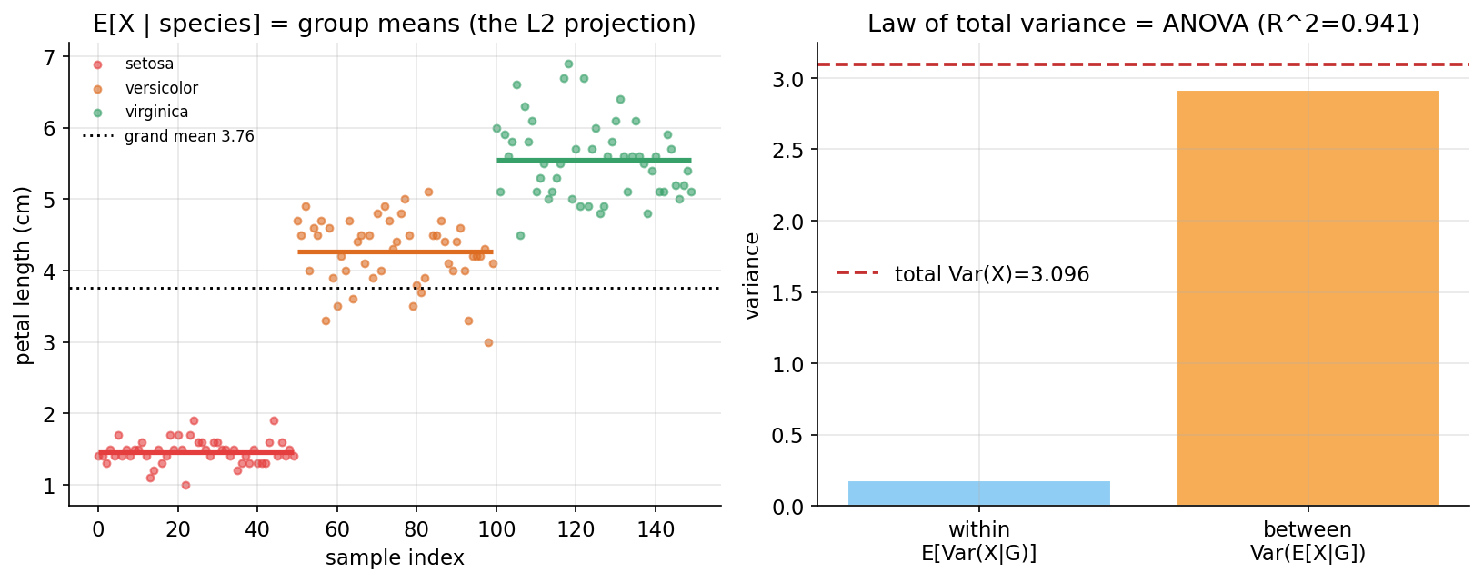
চিত্র: (বামে) iris petal length ও species-ভিত্তিক \(\mathbb E[X\mid\text{species}]\) (group means = L2 projection); (ডানে) within/between variance bar = ANOVA decomposition (\(R^2=0.941\))।
7.8 — Martingales (fair game ও centered co2 increments)
ধারণা। \((M_n)\) martingale যদি \(\mathbb E[M_{n+1}\mid\mathcal F_n]=M_n\) ("ভবিষ্যতের সেরা অনুমান = বর্তমান")। fair \(\pm1\) game-এর partial sum \(S_n\) একটা martingale, তাই \(\mathbb E[S_n]=S_0=0\)। co2 weekly increment center করলে mean-zero \(\varepsilon_t\); তার partial sum \(\approx\) martingale। Doob decomposition: \(X_n=X_0+A_n+M_n\) — predictable trend \(A_n\) (compensator) \(+\) martingale \(M_n\)।
Scratch-এর মূল ধারণা। \(4000\)টি fair-game path-এর partial sum \(S_n\) ও তাদের ensemble-mean; co2 weekly level-এর \(\Delta_t\) center করে \(\varepsilon_t=\Delta_t-\bar\Delta\), তার cumulative sum \(M_t\); predictable trend \(A_t=\) জমা-করা গড়-বৃদ্ধি; reconstruction \(\text{level}_0+A_t+M_t\)।
Demonstrated result (প্রমাণ)। fair game (\(4000\) paths): \(\mathbb E[S_n]\) at \(n{=}100=+0.0270\), \(n{=}400=-0.0720\) (~ \(0\)); table: \(n{=}50\!:-0.099,\ n{=}200\!:+0.000,\ n{=}400\!:-0.072\) (target \(0\))। co2: length \(2225\) (প্রথম \(316.1\), শেষ \(371.5\) ppm); mean weekly drift \(=0.02491\) ppm/week; centered-increment mean \(=2.64\times10^{-17}\), lag-1 corr \(=+0.0862\) (innovation-ঘেঁষা)। Doob: \(\text{level}_0=316.100\), \(A_{\text{end}}=+55.400\) (predictable), \(M_{\text{end}}=-0.000\) (martingale) ⇒ \(316.100+55.400+(-0.000)=371.500=\) actual last (reconstruction error \(=1.76\times10^{-12}\))।
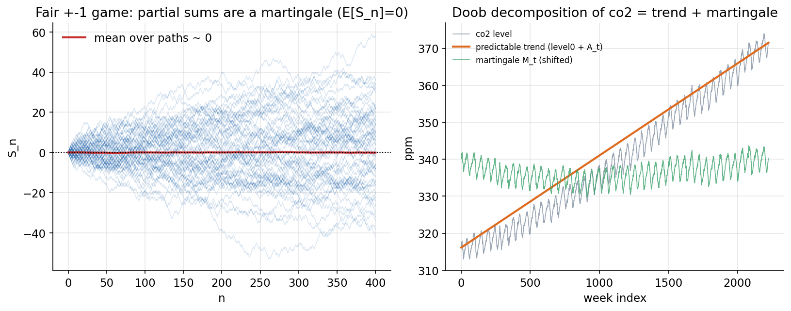
চিত্র: (বামে) fair \(\pm1\) game-এর partial sum path ও তাদের গড় (\(\approx 0\), martingale); (ডানে) co2 level-এর Doob decomposition = predictable trend \(+\) martingale।
7.9 — Martingale convergence (Pólya urn) ও Doob's maximal inequality
ধারণা। Martingale Convergence Theorem: \(L^1\)-bounded martingale প্রায়-নিশ্চিতভাবে একটা (এলোমেলো) limit-এ converge করে। Pólya urn: শুরুতে ১ লাল ১ নীল; তোলা বলের রঙের দুটো ফেরত দাও — red-fraction \(R_n\) একটা bounded \([0,1]\) martingale, converge করে কিন্তু limit random (আসলে Uniform\([0,1]\))। Doob's maximal inequality: nonneg (sub)martingale-এ \(P(\max_{k\le n}M_k\ge\lambda)\le\mathbb E[M_n]/\lambda\)।
Scratch-এর মূল ধারণা। \(300\)টি Pólya-urn path (\(500\) draws)-এর red-fraction; ensemble mean ও final-fraction-এর spread; late-time wobble; running max বনাম Doob bound \(\mathbb E[M_n]/\lambda\)।
Demonstrated result (প্রমাণ)। \(\mathbb E[R_n]\): \(n{=}0\!:0.5000,\ n{=}500\!:0.4997\) (~\(1/2\), martingale-mean preserved); final-fraction sd \(=0.2928\), variance \(=0.0857\) (Uniform\([0,1]\) theory \(0.0833\)); limit quantiles (10/25/50/75/90%) \(=[0.081,0.25,0.513,0.746,0.903]\) (পুরো \([0,1]\)-এ ছড়ানো)। late wobble \(\lvert R_{500}-R_{450}\rvert=0.00439\) (প্রায় থিতু ⇒ converges), অথচ final range \([0.014,0.998]\) (limit random)। Doob: \(\lambda{=}0.6\!:P(\max)=0.653\le 0.833\); \(0.7\!:0.490\le0.714\); \(0.8\!:0.337\le0.625\); \(0.9\!:0.157\le0.555\) — সবই ধরে রাখে।
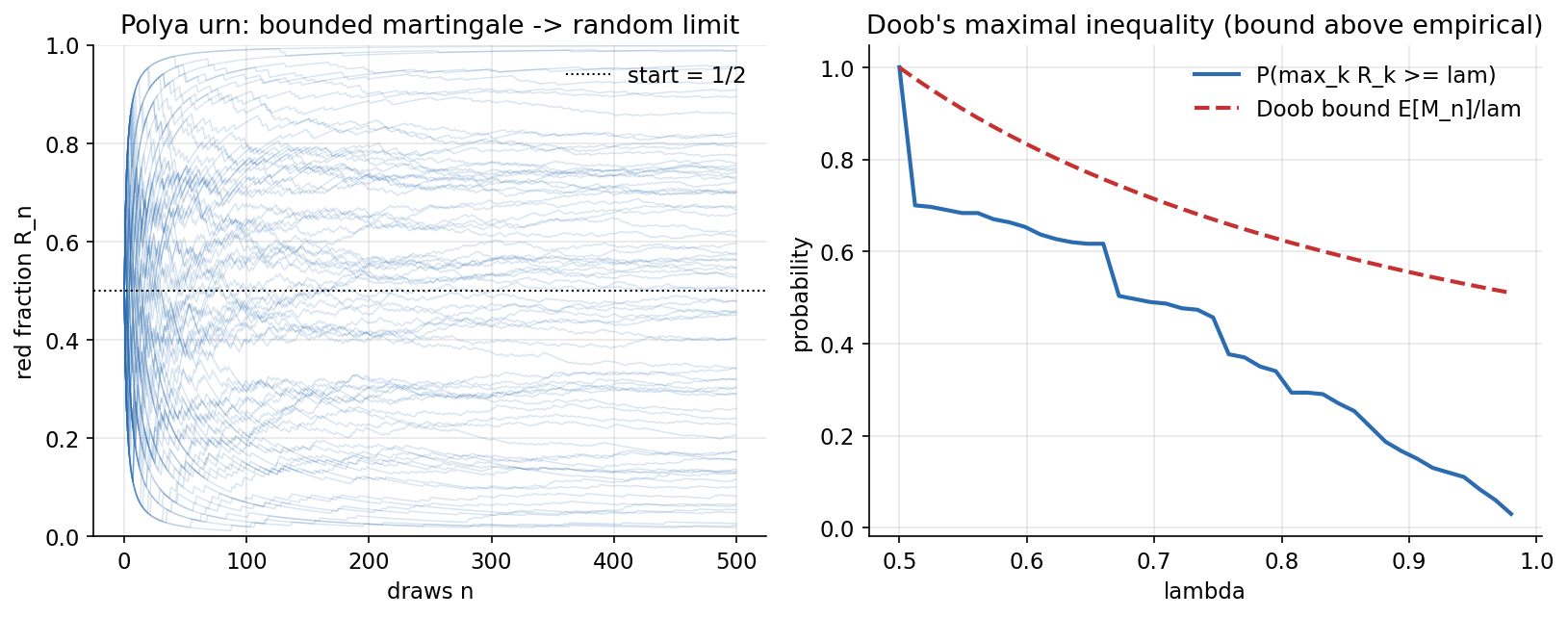
চিত্র: (বামে) Pólya urn red-fraction-এর path আলাদা আলাদা random limit-এ থিতু হয় (bounded martingale converges); (ডানে) \(P(\max\ge\lambda)\) Doob bound \(\mathbb E[M_n]/\lambda\)-এর নিচে থাকে।
7.10 — Characteristic functions ও CLT — capstone
ধারণা। একটা random variable-এর সম্পূর্ণ পরিচয়পত্র characteristic function \(\varphi_X(t)=\mathbb E[e^{itX}]\) — measure-এর Fourier transform, সবসময় থাকে ও আইনকে অদ্বিতীয়ভাবে নির্ধারণ করে; data থেকে estimate empirical CF \(\hat\varphi(t)=\frac1n\sum_k e^{itx_k}\)। Lévy continuity theorem: \(\varphi_{X_n}\to\varphi\) pointwise হলে \(X_n\xrightarrow{d}X\) — এটাই CLT-এর ইঞ্জিন: standardized sample mean \(Z_n=(\bar X_n-\mu)/(\sigma/\sqrt n)\)-এর CF \(\to e^{-t^2/2}\)।
Scratch-এর মূল ধারণা। breast_cancer 'mean area' (skewed) feature-এর standardized single-observation-এর empirical CF \(\hat\varphi(t)\); তারপর resample করে \(Z_n\)-এর empirical CF বিভিন্ন \(n\)-এ; normal CF \(e^{-t^2/2}\)-এর সাথে দূরত্ব \(\sup_t\lvert\hat\varphi_{Z_n}(t)-e^{-t^2/2}\rvert\); আর \(Z_n\)-এর histogram।
Demonstrated result (প্রমাণ)। feature skew \(=1.641\) (right-skewed, \(n=569\)); \(\hat\varphi(0)=1.0000\) (CF at \(0\) সবসময় \(1\)), \(\lvert\hat\varphi(1)\rvert=0.6826\)। \(\lvert\varphi_{Z_n}(1)\rvert\): \(n{=}2\!:0.6522\), \(n{=}50\!:0.6011\) (normal \(e^{-0.5}=0.6065\))। CLT দূরত্ব \(\sup_t\lvert\varphi_{Z_n}-e^{-t^2/2}\rvert\): \(n{=}1\!:0.398,\ 2\!:0.237,\ 5\!:0.129,\ 10\!:0.081,\ 30\!:0.061,\ 100\!:0.016\) — একঘেয়ে সঙ্কুচিত ⇒ \(Z_n\xrightarrow{d}\mathrm N(0,1)\) (Lévy continuity = CLT)।
সম্পূর্ণ ascent, একটি identity-তে
measure (মেজার) থেকে CLT পর্যন্ত পুরো পথ একটাই শৃঙ্খলে বাঁধা — measure (মাপ) \(\to\) integral/expectation (সমাকল/প্রত্যাশা) \(\to\) Fourier transform (characteristic function) \(\to\) convergence in law (আইনে অভিসারণ):
একটা integral (measure-এর সাপেক্ষে expectation) \(n\)-বার গুণ হয়ে limit-এ Gaussian-এ থিতু হয় — এই এক লাইনেই Part VII-এর বিমূর্ত যন্ত্রপাতি বাস্তব data-র সবচেয়ে গভীর নিয়মে রূপ নেয়।
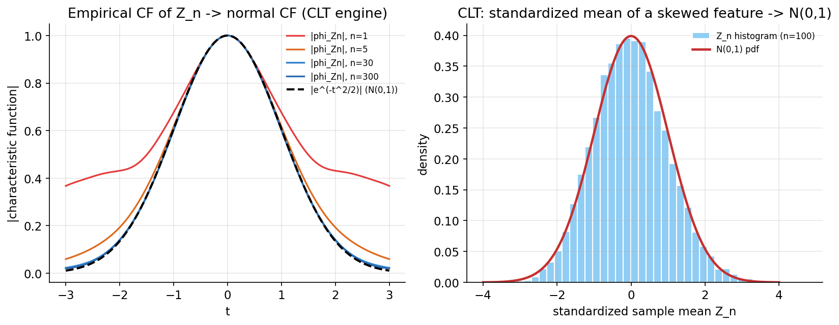
চিত্র: (বামে) \(Z_n\)-এর empirical CF \(\lvert\varphi_{Z_n}(t)\rvert\) যত \(n\) বাড়ে ততই standard-normal CF \(\lvert e^{-t^2/2}\rvert\)-এর দিকে যায় (CLT engine); (ডানে) skewed feature-এর standardized sample mean \(Z_n\)-এর histogram \(\mathrm N(0,1)\) bell curve-এ থিতু হয়।